Regularization for Deep Learning

This is going to be a series of blog posts on the Deep Learning bookwhere we are attempting to provide a summary of each chapter highlighting the concepts that we found to be the most important so that other people can use it as a starting point for reading the chapters, while adding further explanations on few areas that we found difficult to grasp. Please refer this for more clarity on notation.

InMachine Learning, and more so in Deep Learning, overfitting is a major issue that occurs during training. A model is considered as overfitting the training data when the training error keeps decreasing but the test error (or the generalisation error) starts increasing. At this point we tend to believe that the model is learning the training data distribution and not generalising to unseen data. Regularization is a modification we make to the learning algorithm or the model architecture that reduces its generalisation error, possibly at the expense of increased training error. There are various ways of doing this, some of which include restriction on parameter values or adding terms to the objective function, etc.

These constraints are designed to encode some sort of prior knowledge, with a preference towards simpler models to promote generalisation (see Occam’s Razor). The sections present in this chapter are listed below:

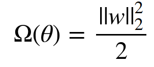
1. Parameter Norm Penalties

The idea here is to limit the capacity (the space of all possible model families) of the model by adding a parameter norm penalty, Ω(θ), to the objective function, J:

Here, θ represents only the weights and not the biases, the reason being that the biases require much less data to fit and do not add much variance.

1.1 L² Parameter Regularization

Here, we have the following parameter norm penalty:

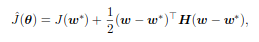
Applying the 2nd order Taylor-Series approximation (ignoring all terms of order greater than 2 in the Taylor-Series expansion) at the point w* (where J̃(θ; X, y) assumes the minimum value, i.e., ∇J̃ (w*)= 0), we get the following expression (as the first order gradient term is 0):

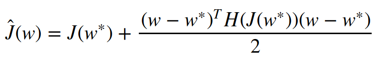
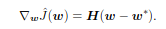
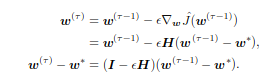
Finally, ∇ Ĵ(w) = H(w — w*) since the first term is just a constant and the derivative of X’ H X (’ represents the transpose) is 2 H X. The overall gradient of the objective function (gradient of Ĵ + gradient of Ω(θ))becomes:

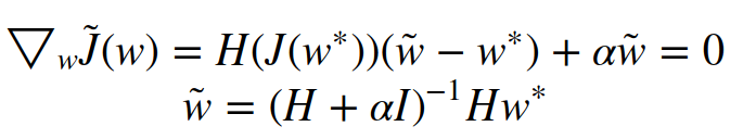
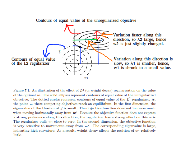
As α approaches 0, w comes closer to w*. Finally, since H is real and symmetric, it can be decomposed into a diagonal matrix ∧ and an orthonormal set of eigenvectors, Q.That is, H = Q’ ∧ Q.

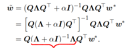
Because of the marked term, the value of each weight is rescaled along the eigenvectors of H. The value of the weights along the eigenvector i,is rescaled by λi /(λi+α), where λi represents the eigenvalue corresponding to that eigenvector.

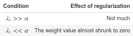
The diagram below illustrates this well:

To look at its application to Machine Learning, we have to look at linear regression. The objective function there is exactly quadratic, given by:

1.2 L¹ parameter regularization

Here, the parameter norm penalty is given by: Ω(θ) = ||w||¹

This makes the gradient of the overall objective function:

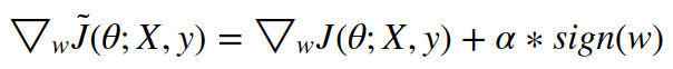
Now, the last term, sign(w), creates some difficulty as the gradient no longer scales linearly with w. This leads to a few complexities in arriving at the optimal solution (details of which can be found in this Appendix notebook):

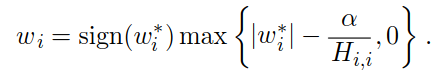
My current interpretation of the max term is that, there shouldn’t be a zero crossing, as the gradient of the absolute value function is not differentiable at zero.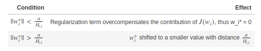

Thus, L¹ regularization has the property of sparsity, which is its fundamental distinguishing feature from L². Hence, L¹ is used for feature selection as in LASSO.

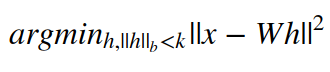
2. Norm penalties as constrained optimization

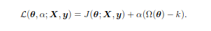
From chapter 4’s section 4, we know that to minimize any function under some constraints, we can construct a generalized Lagrangian function containing the objective function along with the penalties. Suppose we wanted Ω(θ) < k, then we could construct the following Lagrangian:

We get optimal θ by solving the Lagrangian. If Ω(θ) > k, then the weights need to be compensated highly and hence, α should be large to reduce its value below k. Likewise, if Ω(θ)<k, then the norm shouldn’t be reduced too much and hence, α should be small. This is now similar to the parameter norm penalty regularized objective function as both of them encourage lower values of the norm. Thus, parameter norm penalties naturally impose a constraint, like the L²-regularization, defining a constrained L²-ball. Larger α implies a smaller constrained region as it pushes the values really low, hence, allowing a small radius and vice versa. The idea of constraints over penalties is important for several reasons. Large penalties might cause non-convex optimization algorithms to get stuck in local minima due to small values of θ, leading to the formation of so-called dead cells, as the weights entering and leaving them are too small to have an impact. Constraints don’t enforce the weights to be near zero, rather being confined to a constrained region.

Another reason is that constraints induce higher stability. With higher learning rates, there might be a large weight, leading to a large gradient, which could go on iteratively leading to numerical overflow in the value of θ.Constrains, along with reprojection (to the corresponding ball), prevent the weights from becoming too large, thus, maintaining stability.

A final suggestion made by Hinton was to restrict the individual column norms of the weight matrix rather than the Frobenius norm of the entire weight matrix, so as to prevent any hidden unit from having a large weight. The idea here is that if we restrict the Frobenius norm, it doesn’t guarantee that the individual weights would be small, just their norm. So, we might have large weights being compensated by extremely small weights to make the overall norm small. Restricting each hidden unit individually gives us the required guarantee.

3. Regularized & Under-constrained problems

Underdetermined problems are those problems that have infinitely many solutions. A logistic regression problem having linearly separable classes with w as a solution, will always have 2w as a solution and so on. In some machine learning problems, regularization is necessary. For e.g., many algorithms (e.g. PCA) require the inversion of X’ X, which might be singular. In such a case, we can use a regularized form instead. (X’ X + αI) is guaranteed to be invertible.

Regularization can solve underdetermined problems. For e.g. the Moore-Pentose pseudoinverse defined earlier as:

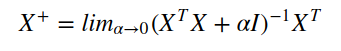
This can be seen as performing a linear regression with L²-regularization.

4. Data augmentation

Having more data is the most desirable thing to improving a machine learning model’s performance. In many cases, it is relatively easy to artificially generate data. For a classification task, we desire for the model to be invariant to certain types of transformations, and we can generate the corresponding (x,y)pairs by translating the input x. But for certain problems, like density estimation, we can’t apply this directly unless we have already solved the density estimation problem.

However, caution needs to be maintained while augmenting data to make sure that the class doesn’t change. For e.g., if the labels contain both “b” and “d”, then horizontal flipping would be a bad idea for data augmentation. Adding random noise to the inputs is another form of data augmentation, while adding noise to hidden units can be seen as doing data augmentation at multiple levels of abstraction.

Finally, when comparing machine learning models, we need to evaluate them using the same hand-designed data augmentation schemes or else it might happen that algorithm A outperforms algorithm B, just because it was trained on a dataset which had more / better data augmentation.

5. Noise Robustness

Noise with infinitesimal variance imposes a penalty on the norm of the weights. Noise added to hidden units is very important and is discussed later in Dropout. Noise can even be added to the weights. This has several interpretations. One of them is that adding noise to weights is a stochastic implementation of Bayesian inference over the weights, where the weights are considered to be uncertain, with the uncertainty being modelled by a probability distribution. It is also interpreted as a more traditional form of regularization by ensuring stability in learning.

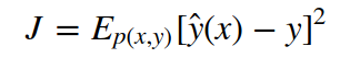
For e.g. in the linear regression case, we want to learn the mapping y(x) for each feature vector x, by reducing the mean square error.

Now, suppose a zero mean unit variance Gaussian random noise, ϵ, is added to the weights. We till want to learn the appropriate mapping through reducing the mean square. Minimizing the loss after adding noise to the weights is equivalent to adding another regularization term which makes sure that small perturbations in the weight values don’t affect the predictions much, thus stabilising training.

Sometimes we may have the wrong output labels, in which case maximizing p(y | x)may not be a good idea. In such a case, we can add noise to the labels by assigning a probability of (1-ϵ) that the label is correct and a probability of ϵ that it is not. In the latter case, all the other labels are equally likely. Label Smoothing regularizes a model with k softmax outputs by assigning the classification targets with probability (1-ϵ ) or choosing any of the remaining (k-1) classes with probability ϵ / (k-1).

6. Semi-Supervised Learning

P(x,y) denotes the joint distribution of x and y, i.e., corresponding to a training sample x, I have a label y. P(x) denotes the marginal distribution of x, i.e., just the training examples without any labels. In Semi-supervised Learning, we use both P(x,y)(some labelled samples) and P(x)(unlabelled samples) to estimate P(y|x)(since we want to predict the class, given the training sample). We want to learn some representation h = f(x)such that samples which are closer in the input space have similar representations and a linear classifier in the new space achieves better generalization error.

Instead of separating the supervised and unsupervised criteria, we can instead have a generative model of P(x) (or P(x, y)) which shares parameters with the discriminative model. The idea is to share the unsupervised/generative criterion with the supervised criterion to express a prior belief that the structure of P(x) (or P(x, y)) is connected to the structure of P(y|x), which is expressed by the shared parameters.

7. Multitask Learning

The idea is to improve the generalization error by pooling together examples from multiple tasks. Similar to how more data leads to more generalization, using a part of the model for different tasks constrains that part to learn good values. There are two types of model parameters:

Task-specific: These parameters benefit only from that particular task.
Generic, shared across all tasks: These are the ones which benefit from learning through various tasks.

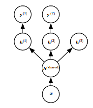
Multitask learning leads to better generalization when there is actually some relationship between the tasks, which actually happens in the context of Deep Learning where some of the factors, which explain the variation observed in the data, are shared across different tasks.

8. Early Stopping

As mentioned at the start of the post, after a certain point of time during training, for a model with extremely high representational capacity, the training error continues to decrease but the validation error begins to increase (which we referred to as overfitting). In such a scenario, a better idea would be to return back to the point where the validation error was the least. Thus, we need to keep calculating the validation metric after each epoch and if there is any improvement, we store that parameter setting. Upon termination of training, we return the last saved parameters.

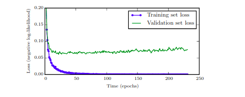
The idea of Early Stopping is that if the validation error doesn’t improve over a certain fixed number of iterations, we terminate the algorithm. This effectively reduces the capacity of the model by reducing the number of steps required to fit the model. The evaluation on the validation set can be done both on another GPU in parallel or done after the epoch. A drawback of weight decay was that we had to manually tweak the weight decay coefficient, which, if chosen wrongly, can lead the model to local minima by squashing the weight values too much. In Early Stopping, no such parameter needs to be tweaked which reduces the number of hyperparameters that we need to tune.

However, since we are setting aside some part of the training data for validation, we are not using the complete training set. So, once Early Stopping is done, a second phase of training can be done where the complete training set is used. There are two choices here:

Train from scratch for the same number of steps as in the Early Stopping case.
Use the weights learned from the first phase of training and retrain using the complete data.

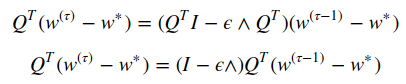
Other than lowering the number of training steps, it reduces the computational cost also by regularizing the model without having to add additional penalty terms. It affects the optimization procedure by restricting it to a small volume of the parameter space, in the neighbourhood of the initial parameters. Suppose 𝛕 and ϵ represent the number of iterations and the learning rate respectively. Then, ϵ𝛕 effectively represents the capacity of the model. Intuitively, this can be seen as the inverse of the weight decay co-efficient λ. When ϵ𝛕 is small (or λ is large), the parameter space is small and vice versa. This equivalence holds true for a linear model with quadratic cost function (initial parameters w⁰ = 0). Taking the Taylor Series Approximation of J(w) around the empirically optimal weights w*:

multiplying with Q’ on both sides and using the fact that Q’Q = I (Q is orthonormal):

Assuming ϵ to be small enough:

The equation for L² regularization is given by:

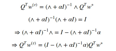
Thus, if the hyperparameters are such that:

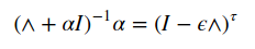
L²-regularization can be seen as equivalent to Early Stopping.

9. Parameter Tying and Parameter Sharing

Till now, most of the methods focused on bringing the weights to a fixed point, e.g. 0 in the case of norm penalty. However, there might be situations where we might have some prior knowledge on the kind of dependencies that the model should encode. Suppose, two models A and B, perform a classification task on similar input and output distributions. In such a case, we’d expect the parameters for both the models to be similar to each other as well. We could impose a norm penalty on the distance between the weights, but a more popular method is to force the set of parameters to be equal. This is the essence behind Parameter Sharing. A major benefit here is that we need to store only a subset of the parameters (e.g. storing only the parameters for model A instead of storing for both A and B) which leads to large memory savings. In the example of Convolutional Neural Networks or CNNs (discussed in Chapter 9), the same feature is computed across different regions of the image and hence, a cat is detected irrespective of whether it is at position ior i+1 .

10. Sparse Representations

We can place penalties on even the activation values of the units which indirectly imposes a penalty on the parameters. This leads to representational sparsity, where many of the activation values of the units are zero. In the figure below, h is a representation of x, which is sparse. Representational sparsity is obtained similarly to the way parameter sparsity is obtained, by placing a penalty on the representation h instead of the weights.

Another idea could be to average the activation values across various examples and push it towards some value. An example of getting representational sparsity by imposing hard constraint on the activation value is the Orthogonal Matching Pursuit (OMP) algorithm, where a representation h is learned for the input x by solving the constrained optimization problem:

where the constraint is on the the number of non-zero entries. The problem can be solved efficiently when W is restricted to be orthogonal

11. Bagging and Other Ensemble Methods

The techniques which train multiple models and take the maximum vote across those models for the final prediction are called ensemble methods. The idea is that it’s highly unlikely that multiple models would make the same error in the test set.

Suppose that we have K regression models, with the model #i making an error ϵi on each example, where ϵi is drawn from a zero mean, multivariate normal distribution such that: 𝔼(ϵi²)=v and 𝔼(ϵiϵj)=c. The error on each example is then the average across all the models: (∑ ϵi)/K.

The mean of this average error is 0 (as the mean of each of the individual ϵiϵi is 0). The variance of the average error is given by:

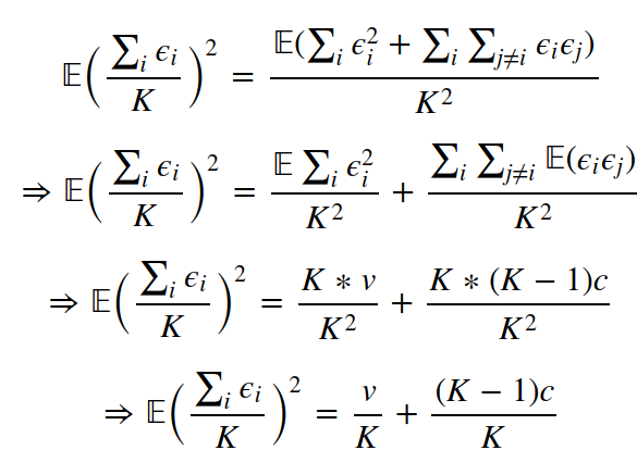
Thus, if c = v, then there is no change. If c = 0, then the variance of the average error decreases with K. There are various ensembling techniques. In the case of Bagging (Bootstrap Aggregating), the same training algorithm is used multiple times. The dataset is broken into K parts by sampling with replacement (see figure below for clarity) and a model is trained on each of those K parts. Because of sampling with replacement, the K parts have a few similarities as well as a few differences. These differences cause the difference in the predictions of the K models. Model averaging is a very strong technique.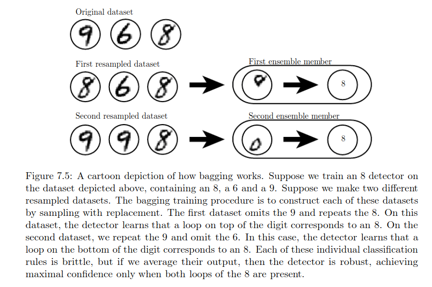

12. Dropout

Dropout is a computationally inexpensive, yet powerful regularization technique. The problem with bagging is that we can’t train an exponentially large number of models and store them for prediction later. Dropout makes bagging practical by making an inexpensive approximation. In a simplistic view, dropout trains the ensemble of all sub-networks formed by randomly removing a few non-output units by multiplying their outputs by 0. For every training sample, a mask is computed for all the input and hidden units independently. For clarification, suppose we have h hidden units in some layer. Then, a mask for that layer refers to a h dimensional vector with values either 0(remove the unit) or 1(keep the unit).

There are a few differences from bagging though:

In bagging, the models are independent of each other, whereas in dropout, the different models share parameters, with each model taking as input, a sample of the total parameters.
In bagging, each model is trained till convergence, but in dropout, each model is trained for just one step and the parameter sharing makes sure that subsequent updates ensure better predictions in the future.

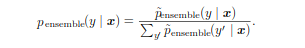
At test time, we combine the predictions of all the models. In the case of bagging with K models, this was given by the arithmetic mean. In case of dropout, the probability that a model is chosen is given by p(μ), with μ denoting the mask vector. The prediction then becomes ∑ p(μ)p(y|x, μ). This is not computationally feasible, and there’s a better method to compute this in one go, using the geometric mean instead of the arithmetic mean.

We need to take care of two main things when working with geometric mean:

None of the probabilities should be zero.
Re-normalization to make sure all the probabilities sum to 1.

The advantage for dropout is that first term can be approximated in one pass of the complete model by dividing the weight values by the keep probability (weight scaling inference rule). The motivation behind this is to capture the right expected values from the output of each unit, i.e. the total expected input to a unit at train time is equal to the total expected input at test time. A big advantage of dropout then is that it doesn’t place any restriction on the type of model or training procedure to use.

Points to note:

Reduces the representational capacity of the model and hence, the model should be large enough to begin with.
Works better with more data.
Equivalent to L² for linear regression, with different weight decay coefficient for each input feature.

Biological Interpretration:

During sexual reproduction, genes could be swapped between organisms if they are unable to correctly adapt to the unusual features of any organism. Thus, the units in dropout learn to perform well regardless of the presence of other hidden units, and also in many different contexts.

Adding noise in the hidden layer is more effective than adding noise in the input layer. For e.g. let’s assume that some unit learns to detect a nose in a face recognition task. Now, if this unit is removed, then some other unit either learns to redundantly detect a nose or associates some other feature (like mouth) for recognising a face. In either way, the model learns to make more use of the information in the input. On the other hand, adding noise to the input won’t completely removed the nose information, unless the noise is so large as to remove most of the information from the input.

13. Adversarial Training

Deep Learning has outperformed humans in the task of Image Recognition, which might lead us to believe that these models have acquired a human-level understanding of an image. However, experimentally searching for an x′(given an x), such that prediction made by the model changes, shows otherwise. As shown in the image below, although the newly formed image (adversarial image) looks almost exactly the same to a human, the model classifies it wrongly and that too with very high confidence:

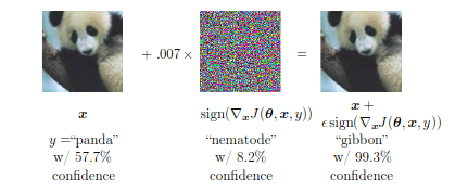
Adversarial training refers to training on images which are adversarially generated and it has been shown to reduce the error rate. The main factor attributed to the above mentioned behaviour is the linearity of the model (say y = Wx), caused by the main building blocks being primarily linear. Thus, a small change of ϵ in the input causes a drastic change of Wϵ in the output. The idea of adversarial training is to avoid this jumping and induce the model to be locally constant in the neighborhood of the training data.

This can also be used in semi-supervised learning. For an unlabelled sample x, we can assign the label ŷ (x) using our model. Then, we find an adversarial example, x′, such that y(x′)≠ŷ (x) (an adversary found this way is called virtual adversarial example). The objective then is to assign the same class to both x and x′. The idea behind this is that different classes are assumed to lie on disconnected manifolds and a little push from one manifold shouldn’t land in any other manifold.

14. Tangent Distance, Tangent Prop and manifold Tangent Classifier

Many ML models assume the data to lie on a low dimensional manifold to overcome the curse of dimensionality. The inherent assumption which follows is that small perturbations that cause the data to move along the manifold (it originally belonged to), shouldn’t lead to different class predictions. The idea of the tangent distance algorithm to find the K-nearest neighbors using the distance metric as the distance between manifolds. A manifold Mi is approximated by the tangent plane at Xi, hence, this technique needs tangent vectors to be specified.

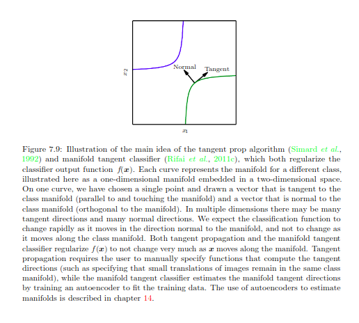
The tangent prop algorithm proposed to learn a neural network based classifier, f(x), which is invariant to known transformations causing the input to move along its manifold. Local invariance would require that ▽ f(x) is perpendicular to the tangent vectors V(i). This can also be achieved by adding a penalty term that minimizes the directional directive of f(x) along each of the V(i).

It is similar to data augmentation in that both of them use prior knowledge of the domain to specify various transformations that the model should be invariant to. However, tangent prop only resists infinitesimal perturbations while data augmentation causes invariance to much larger perturbations.

Manifold Tangent Classifier works in two parts:

Use Autoencoders to learn the manifold structures using Unsupervised Learning.
Use these learned manifolds with tangent prop.

I have missed out on many details along the way in the trade-off for explaining the ones I found the most relevant today. If you’re looking for the summary of previous chapters or are more comfortable reading from a Jupyter Notebook, feel free to have a look over our repository here. If you are interested in reading more such summaries and/or receiving research paper implementations/explanations, follow our publication, Inveterate Learner. Finally, I thank my co-author for the publication, Ameya Godbole, for reviewing the post and doing several important corrections.

by Adrian Rosebrock

The recent thought

Monday, June 4, 2018