A modified Artificial Bee Colony algorithm to solve Clustering problems

A step-by-step implementation in Python,

Now it’s time for putting our hands on some real data and explain how we can use our Python implementation of the ABC algorithm to perform the clustering task. But before that, let’s get a little deeper into the clustering problem.

The Clustering Problem

The clustering problem is a non-well-defined NP-hard problem where the basic idea is to find hidden patterns in our data. There is not a formal definition of what is a cluster, but it’s associated with the idea of grouping elements in such a way that we can differentiate elements in distinct groups.

There are different families of algorithms that define the clustering problem in distinct ways. A classical way to define the clustering problem, often seen in literature, is to reduce it to a mathematical problem known as finding a k-partition of the original data.

Finding a k-partition of a set S, is defined as finding k subsets of S, that obeys two rules:

• The intersection of any distinct of those subsets is equal to the empty set.
• The union of all k subsets is equal to S.

Basically, at the end of this partitional clustering procedure, we want to find distinct subsets of our original dataset, in such a way that, no instance will belong to more than one group. This can be illustrated on the image below:

On the left the original data, on the right the partitioned data with k=2.

An example of how centroids can be used to perform a data partition with k=2.

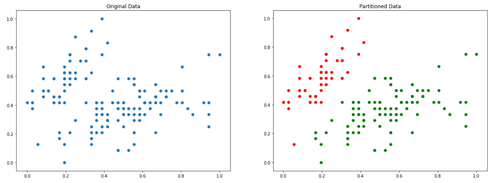
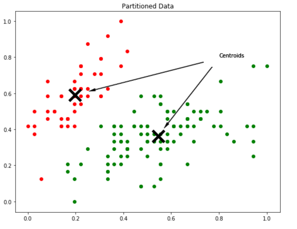
How can we split the data to perform the partition illustrated in the above image? Well, the output of the clustering procedure is a set of centroids. Centroids are basically the representative entities of each group, so if we want a k-partition of our data, then we will have k centroids.

The centroids are also points on the search space defined by our data, and since each centroid defines a group, each data point will be assigned to the closest centroid from it.

Modifying the Artificial Bee Colony for Clustering

Well, now that we know what is the clustering problem, how can we modify the original ABC algorithm to perform such task ? Guess what, we don’t! Yes, that is what you just read, we don’t have to modify our ABC implementation at all. The only thing we have to do is look to the clustering problem and turn it into an optimization task! But how can we do that ?

As we saw on the previous article, a well defined optimization problem needs a search space, a set o d-dimensional input decision variables and an objective function. If we look at each bee in our artificial colony as a whole solution for our clustering problem, than each bee can represent a complete set of candidate centroids! If we are working on a d-dimensional space, and we want to perform a k-partition on our dataset, then each bee will be a k·d-dimensional vector!

Awesome! Now that we have defined how to represent our input decision variables, we just have to figure out how to define the boundaries of our search space and what will be our objective function.

The boundaries of our search space are easy, we can normalize our entire dataset with the [0, 1] interval, and define our objective function as having the boundaries from 0 to 1. Done, that’s it. Now let’s go to a more complicated part: How to define our objective function?

In the partitional clustering approach, we want to maximize the distance between two distinct groups, and minimize the inner distance within a group. There are several objective functions that are used in the literature, but the most well-known and used it’s called Sum of Squared Errors (SSE).

Formula for the Sum of Squared Errors. Don’t be afraid, is not that scary.

What does this formula means? Well, the Sum of Squared Errors (SSE) is a clustering metric, and the idea behind it is very simple. It’s basically a numerical value that computes the squared distance of each instance in our data to its closest centroid. The goal of our optimization task will be to minimize this function.

We can use our previous framework of objective functions to implement the Sum of Squared Errors as follows:

Hands On with some Real Data

It’s time to put our hands on some real data and test how well our ABC algorithm for clustering can perform. For this study case, we are going to use the well-known Iris Dataset.

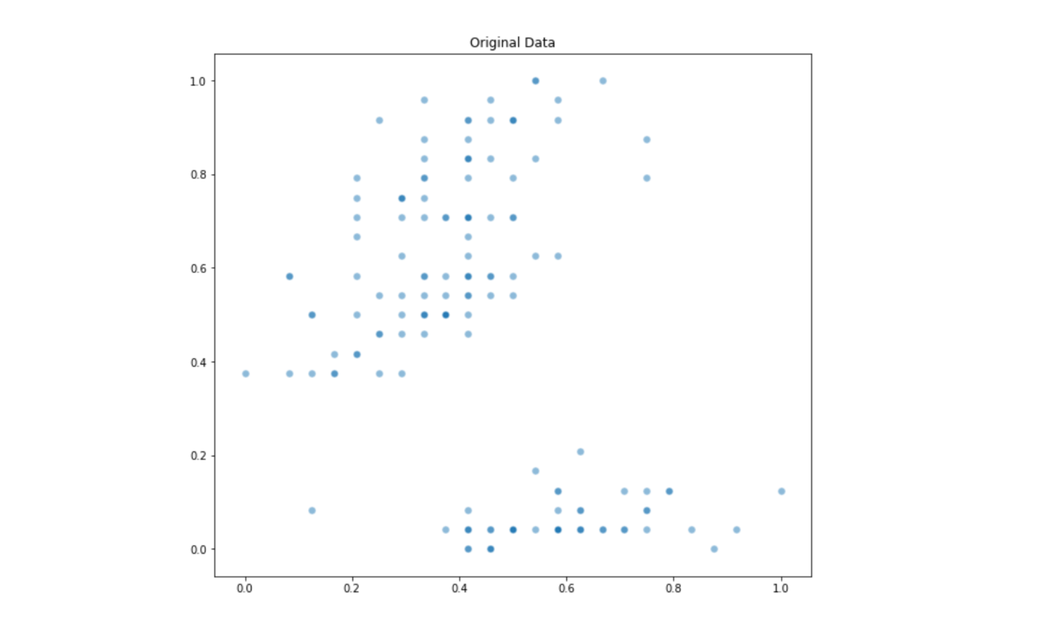
This is an originally 4-dimensional dataset which includes characteristics from three kinds of plants. For visualization purposes, we will be using only two dimensions of this dataset. Let’s check the relationship between the second and fourth dimension of this dataset:

The output from the above code can be seen bellow:

The original data distribution.

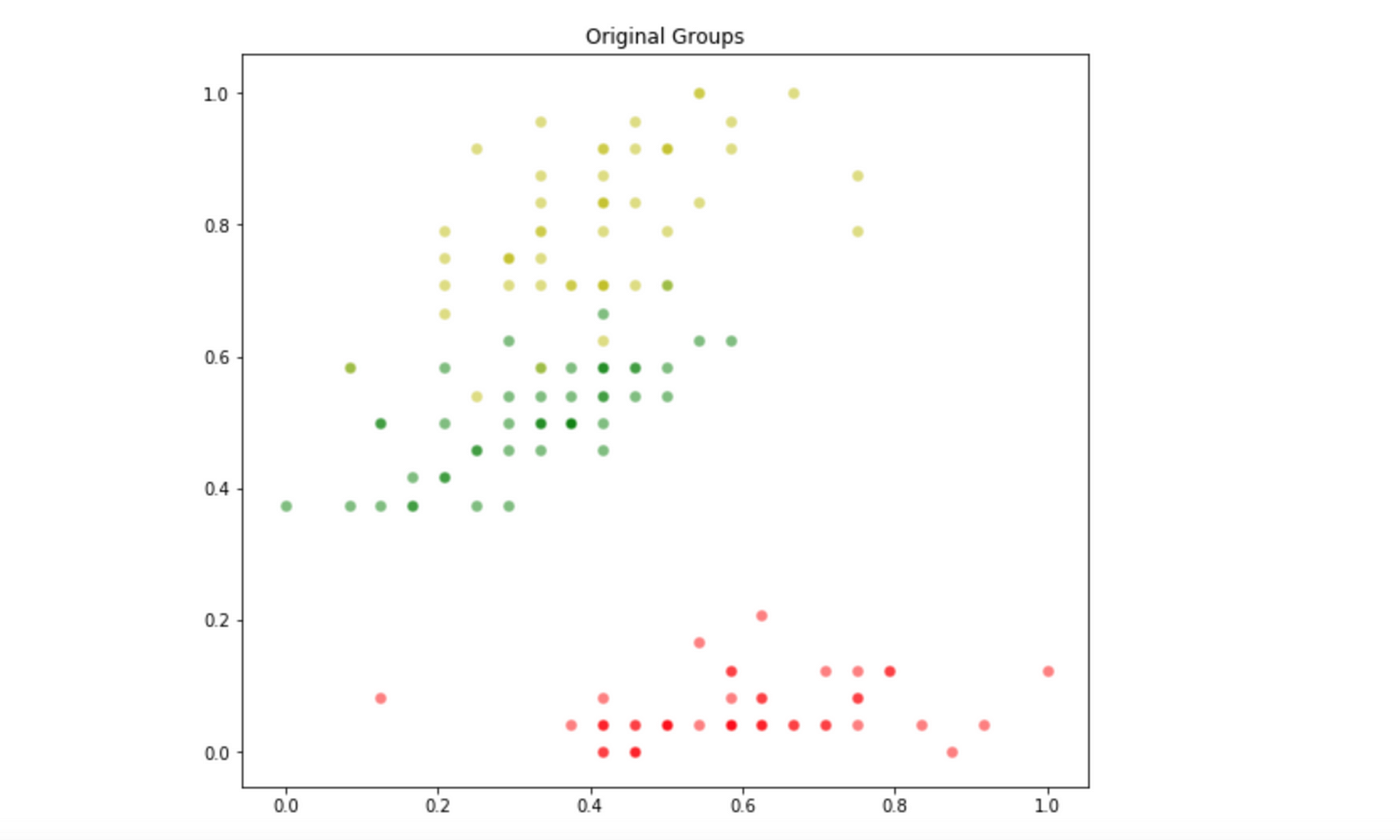
Since we will be using this data as a benchmark test, we already know what is the optimal partition of it, and its given by the original distribution of the three types of flower. We can visualize the original optimal partition of theIris Dataset with the following Python code:

Which plot the following distribution:

The original groups within our dataset

Now that we know what is the original optimum partition for this sample data, it’s time to find out if our ABC algorithm is able to find a very close solution for this problem. We are going to use our Sum of Squared Errorsobjective function, and set the number of partitions to three.

Since the initialization is random, it’s very likely that the order of the generated centroids does not match with the order of classes. Because of that, when plotting our output for the ABC algorithm the colors for the groups may not match. That’s not really important, what we will actually will look is how well the correspondent partitioned groups will look.

The output of our Python code can be seen bellow:

The partition of our dataset found by the ABC algorithm.

Whoa, that’s awesome! If we take a look on the original partition and the one generated by our ABC algorithm, we can see that it was able to find a partition really close the optimal. That proves how powerful is the “modified” ABC algorithm for clustering. We can also take a look on how the optimization process went by looking at the optimality_tracking attribute of our ABC algorithm:

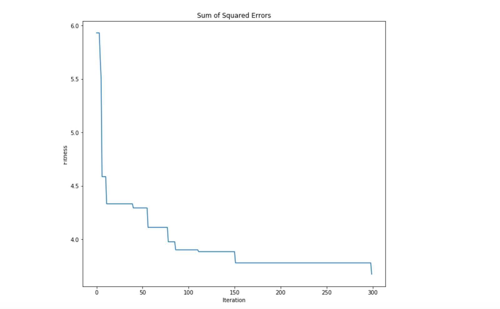
As expected, the ABC algorithm was really efficient in minimizing the SSEobjective function. We can see that Swarm Intelligence posses some powerful machinery for solving optimization problems, an adapt those algorithms to solve real-world problems is just a matter of how we can reduce those problems into an optimization task.