NEW OPTIMIZATION FUNCTIONS IN PYTHON

Hi all again! In one of my posts in the end of last year I mentioned optimization as one of the most interesting field for machine learning researchers. I am a huge fan of numerical optimization since my bachelor degree and I decided to recap some basics first of all for myself and tell you, guys, some recipes on how to solve optimization problems for machine learning and not only.

I want to start with simple functions optimization, after move on to more complex functions with several local minimums or that are just difficult to find minima in, constrained optimization and geometrical optimization problems. I also want to use totally different methods for optimization: starting with gradient based methods and finishing with evolutionary algorithms and latest ideas from deep learning battlefront. Of course, machine learning applications will go alongside, but the real goal is to show big landscape of problems and algorithms in numerical optimization and to give you understanding, what’s really happening inside your favorite AdamOptimizer().

Another moment, that I personally like a lot: I want to concentrate on visualizations of different algorithms behavior to understand intuition behind math and code, so in this series of posts there will be a lot of GIFs — for zero order methods, first order in SciPy, first order in Tensorflow and second order methods. As always, I strongly recommend you to check out source code too.

Functions for optimization

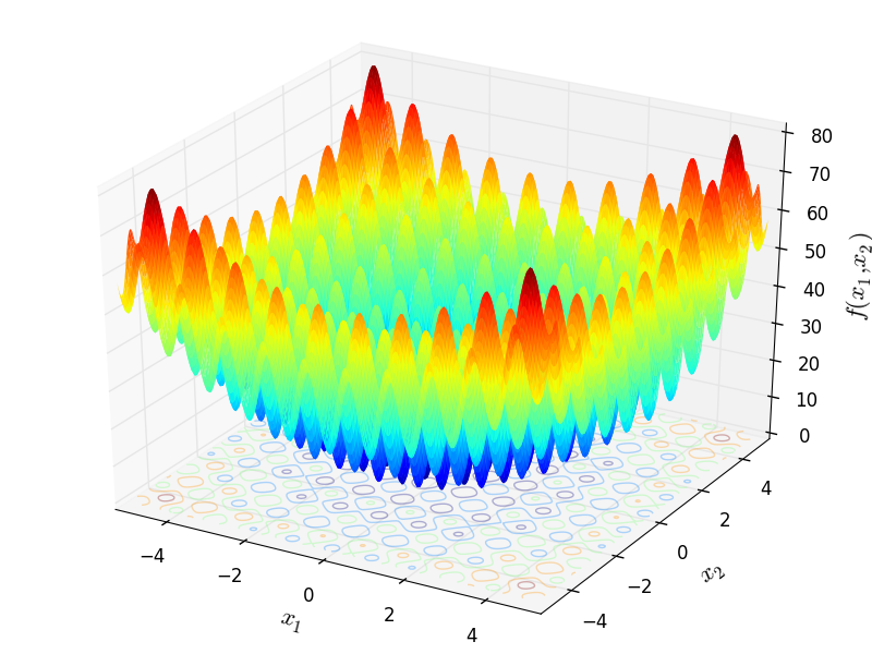
First of all, let’s define set of functions for today. I decided to start with the simplest ones, that supposed to be very easy to optimize and to show general walkthrough with different tools. The whole list of functions and formulas you can find here, I just chose some of them. I also need to notice, that code for visualization is used from this amazing tutorial.

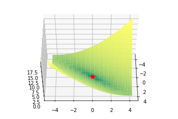
Bowl functions

Bohachevsky function and Trid functions

def bohachevsky(x, y):
    return x**2 + 2*y**2 - 0.3*np.cos(3*3.14*x) -     0.4*np.cos(4*3.14*y) + 0.7

def trid(x, y):
    return (x-1)**2 + (y-1)**2 - x*y

Bohachevsky function (on the left) and Trid function (on the right)

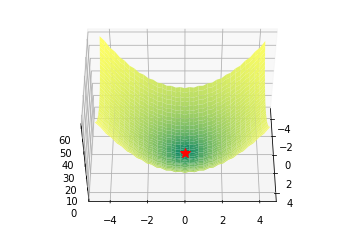
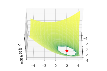
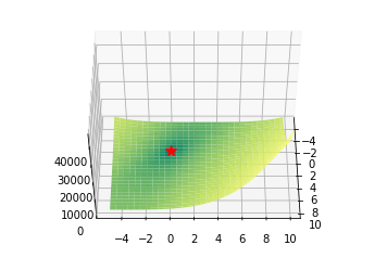
Plate functions

Booth, Matyas and Zakharov functions

def booth(x, y):
    return (x + 2*y - 7)**2 + (2*x + y - 5)**2

def matyas(x, y):
    return 0.26*(x**2 + y**2) - 0.48*x*y

def zakharov(x, y):
    return (x**2 + y**2) + (0.5*x + y)**2 + (0.5*x + y)**4

Booth (left), Matyas (center) and Zakharov (right) functions

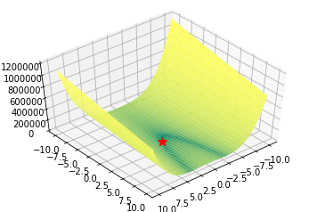
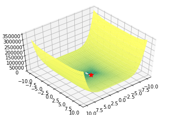
Valley functions

Rozenbrock, Beale and Six Hump Camel functions

def rozenbrock(x, y):
    return (1-x)**2 + 100*(y - x**2)**2

def beale(x, y):
    return (1.5 - x + x*y)**2 + (2.25 - x + x*y**2)**2 + (2.65 - x + x*y**3)**2

def six_hump(x, y):
    return (4 - 2.1*x**2 + x**4/3)*x**2 + x*y + (-4 + 4*y**2)*y**2

Rozenbrock (left), Beale (center) and Six Hump Camel (right) functions

Algorithms

In this article we will review just basic algorithms for optimization from SciPy and Tensorflow.

Optimization without gradients

Very often our cost function is noisy, or non-differentiable, and, hence, we can’t apply methods that use gradient in this case. In this tutorial we compare Nelder-Mead and Powell algorithms as ones, that don’t compute gradients. First approach builds (n+1)-dimensional simplex and finds a minimum on it, sequentially updating the simplex. Powell method makes one-dimensional search on each of the basis vectors of the space. We use SciPy implementations for them:

minimize(fun, x0, method='Nelder-Mead', tol=None, callback=make_minimize_cb)

Callback is used for saving intermediate results, taken from here, check the full code on my Github. Read more about Nelder-Mead and Powell methods.

First order algorithms

This family of algorithms you probably know much better from machine learning frameworks like Tensorflow. The idea behind all of them is moving in direction of anti-gradient that leads to the minima of the function. But the details of moving to this minima differ a lot. We will review the following from Tensorflow: Gradient descent with momentum (and without), Adam and RMSProp. For TF we will define functions like this (whole code is here):

x = tf.Variable(8., trainable=True)
y = tf.Variable(8., trainable=True)

f = tf.add_n([
    tf.add(tf.square(x), tf.square(y)), 
    tf.square(tf.add(tf.multiply(0.5, x), y)), 
    tf.pow(tf.multiply(0.5, x), 4.)   
])

and optimize them following way:

opt = tf.train.GradientDescentOptimizer(0.01)
grads_and_vars = opt.compute_gradients(f, [x, y])
clipped_grads_and_vars = [(tf.clip_by_value(g, xmin, xmax), v) for g, v in grads_and_vars]

train = opt.apply_gradients(clipped_grads_and_vars)

sess = tf.Session()
sess.run(tf.global_variables_initializer())

points_tf = []
for i in range(100):
    points_tf.append(sess.run([x, y]))
    sess.run(train)

From SciPy we will use Conjugated Gradient, Newton Conjugated Gradient, Truncated Newton, Sequential Least Squares Programmingmethods. You can read more about this kind of algorithms in a free online book by Stephen Boyd and Lieven Vandenberghe. Another cool comparison of optimization for machine learning is in this blog post.

The SciPy API is more or less the same as with zero-order methods, you can check it here.

Second order algorithms

We also will touch couple of algorithms that use second order derivatives for faster convergence: dog-leg trust-region, nearly exact trust-region. These algorithms sequentially solve sub-optimization tasks, where regions of search (usually spheres) are being found. As we know, these algorithms require a Hessian (or its approximation), so we will use numdifftools library to compute them and pass into SciPy optimizer (inspired by click, whole code click):

from numdifftools import Jacobian, Hessian

def fun(x):
    return (x[0]**2 + x[1]**2) + (0.5*x[0] + x[1])**2 + (0.5*x[0] + x[1])**4

def fun_der(x):
    return Jacobian(lambda x: fun(x))(x).ravel()

def fun_hess(x):
    return Hessian(lambda x: fun(x))(x)

minimize(fun, x0, method='dogleg', jac=fun_der, hess=fun_hess)

Optimization without gradients

In this post I want to evaluate results first of all from visual point of view, I believe that it’s very important to see with your eyes trajectories first and after all the formulas will be much more clear.

Here are just some of the visualizations, you can find more on this Imgur.

Bohachevsky, Matyas and Trid functions are optimized with Nelder-Mead and Powell

Optimization with Jacobian

Here you can see comparison of gradient based methods from SciPy and Tensorflow, more GIFs are here and here. Some of these algorithms may look too “slow”, but it depends a lot on the choice of hyperparameters, we take a look on them a bit later.

Booth, Rosenbrok and Six Hump functions in SciPy

Booth, Rosenbrok and Six Hump functions in Tensorflow

Optimization with Hessian

Using second derivative almost immediately leads us to the minima for “good” looking quadratic functions, but it’s not that simple for other… for example for Bohachevsky function it comes close to the minima, but not exactly there. More examples (also diverging!) of other functions are here.

Bohachevsky, Matyas and Trid functions optimization trajectories

Notes on hyperparameters

Learning rate

First of all, I think you have noticed, that such popular adaptive algorithms as Adam and RMSprop were very slow comparing even to SGD, but they were designed to be faster? This is because of the too small learning rate exactly for these loss surfaces. This parameter has to be tuned for each problem separately. On the images below you can see what happens if we increase it to the values of 1.

Increased learning rate for Adam and RMSProp

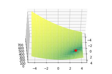
Starting point

Usually we just start search of minima from a random point (or with some smart initializers like in neural networks), but in general it’s not correct strategy. On the example below you can see, how even second order methods can diverge if started from the wrong point. One of the ways to overcome this issue in pure optimization problem is use of global search algorithms to estimate area of global minima (we will do it later).

Diverging second order methods from the wrong starting point

Notes on machine learning

Most probably, right now you want to try some of SciPy algorithms to train your machine learning models in Tensorflow. You even don’t need to build a custom optimizer, because tf.contrib.opt already has it for you! It allows to use the same algorithms and their parameters:

vector = tf.Variable([7., 7.], 'vector')

# Make vector norm as small as possible.
loss = tf.reduce_sum(tf.square(vector))

optimizer = ScipyOptimizerInterface(loss, options={'maxiter': 100}, method='SLSQP')

with tf.Session() as session:
  optimizer.minimize(session)

Conclusion

This article is just introduction to the field of optimization, but even from these results we can see, that it’s not easy at all. Using “cool” second order or adaptive rate algorithms doesn’t guarantee to us convergence to the minima, moreover, we have some hyperparameters as learning rate and starting point to find. Anyway, now you have some intuition, of how all these algorithms work. For example, you can be sure that it’s good idea to use second order methods for quadratic-like functions or not to be shy to use algorithms, that doesn’t require derivatives, they also work well and must be part of your optimization arsenal.

We also need to remember, that these functions were not really difficult at all! What will happen when we will encounter something like this… with constraints… and stochasticity?

Rastrigin function