Neural networks for algorithmic trading: backtesting in Pandas

Hi all again! If you’re reading my blog regularly you know that I have published a bunch of tutorials on financial time series forecasting using neural networks. If you’re here for the first time, here is the list of them:

We were mostly concentrated on forecasting accuracy and experimenting around that before and we touched backtesting issue very briefly and using code from the Mike Halls-Moore’s book. Of course having a nice backtesting code allows to build really good strategies with risk management, money management and consider different scenarios, but if you’re researching just signals obtained from different data sources (even it’s just historical prices) with use of machine learning you need something simpler to understand if these signals to go long or short are really useful. Basically we just want to check the difference between prices and multiply it by signal sign — up or down and accumulate this info during test period.

It can be very easily done with Pandas! I borrowed the code basis again from Mike Halls-Moore QuantStart, but changed it for our purposes. Code used in this tutorial you can check in my Github.

Backtesting scenario

Let’s assume we want to trade Litecoin cryptocurrency starting from 1 January of 2018 using neural network based indicators and compare this performance to the scenario when we just invested in it (buy and hold strategy). First we will train a neural network on daily data from 2015 to 2017. After we will prepare the signals and backtest it. As you can see, holding this coin from historical perspective doesn’t look as a good idea, but let’s see if we can outperform this with machine learning.

Data loading

First I have downloaded daily data of LTC from 01.01.2015 to 10.03.2018 using API of https://www.coinapi.io, they have free option for small amount of data, which we be enough to test our hypothesis though.

Now we need to load data and split it into train and test data samples:

symbol = 'LTC1518'
bars = pd.read_csv('./data/%s.csv' % symbol, header=0, parse_dates=['Date'])

START_TRAIN_DATE = '2015-01-01'
END_TRAIN_DATE = '2017-12-31'
START_TEST_DATE = '2018-01-01'
END_TEST_DATE = '2018-03-09'

train_set = bars[(bars['Date'] > START_TRAIN_DATE) & (bars['Date'] < END_TRAIN_DATE)]
test_set = bars[(bars['Date'] > START_TEST_DATE) & (bars['Date'] < END_TEST_DATE)]

After this we simply loop over this data (OHLCV) with some window (I have chosen 7 days) to create data samples and took next day change sign to create labels (code is here) and after created train and test data sets:

X_train, Y_train = create_dataset(train_set)
X_test, Y_test = create_dataset(test_set)

Training a neural network

Just for educational purposes we will create very simple model which will be a perceptron, but “on steroids”: we will augment it with noise regularization, dropout, batch normalization of the inputs and train the model correctly:

def get_lr_model(x1, x2):
    main_input = Input(shape=(x1, x2, ), name='main_input')
    x = GaussianNoise(0.01)(main_input)
    x = Flatten()(x)
    x = BatchNormalization()(x)
    x = Dropout(0.5)(x)
    output = Dense(1, activation = "sigmoid", name = "out")(x)
    final_model = Model(inputs=[main_input], outputs=[output])
    final_model.compile(optimizer=Adam(lr=0.001, amsgrad=True),  loss='binary_crossentropy', metrics = ['accuracy'])
    return final_model

I am adding gaussian noise to the input on purpose — it must work as some kind of regularization and data augmentation — neural network is supposed to learn to ignore this noise (what a calembour — noise data augmented by artificial noise) and learn representative features.

reduce_lr = ReduceLROnPlateau(monitor='val_loss', factor=0.9, patience=50, min_lr=0.000001, verbose=0)
checkpointer = ModelCheckpoint(filepath="test.hdf5", verbose=0, save_best_only=True)
es = EarlyStopping(patience=100)

model = get_lr_model(X_train.shape[1], X_train.shape[-1])

history = model.fit(X_train, Y_train, 
              epochs = 1000, 
              batch_size = 64, 
              verbose=0, 
              validation_data=(X_test, Y_test),
              callbacks=[reduce_lr, checkpointer, es],
              shuffle=True)

After training I am checking the most informative metics for binary classification as confusion matrix, precision, recall and Matthews correlation coefficient (everything is in scikit-learn):

pred = [1 if p > 0.5 else 0 for p in pred]
C = confusion_matrix(Y_test, pred)

print matthews_corrcoef(Y_test, pred)
print(C / C.astype(np.float).sum(axis=1))
print classification_report(Y_test, pred)
print '-' * 20

The results are following:

MATTHEWS CORRELATION
0.17021289926939803
CONFUSION MATRIX
[[0.42857143 0.53333333]
 [0.28571429 0.73333333]]
CLASSIFICATION REPORT
             precision    recall  f1-score   support

          0       0.60      0.43      0.50        28
          1       0.58      0.73      0.65        30

avg / total       0.59      0.59      0.58        58

And accuracy/loss plots look like this:

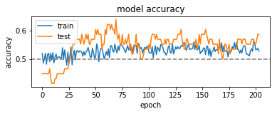
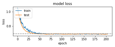
which most probably can mean that we can really predict something on our test period, but let’s check how it will trade!

Preparing signals

This part is simple and tricky same time. First we will change outputs to {-1, 1} as signs of direction of market price movement.

pred = [1 if p == 1 else -1 for p in pred]

Next we want to consider situation when we predict change not for a single day ahead, but for 2, 3 or the whole week. For the strategy it will mean that we long or short on the day X and after wait a week without making any trades — for these days we will say that signal is 0:

pred = [p if i % FORECAST == 0 else 0 for i, p in enumerate(pred)]

After, we want to do everything nicely with Pandas, so if we want to subtract price of the target day (let’s say tomorrow) from the price of buying/selling day (let’s say today) we need to shift the target day column for the period of the forecast back:

test_set['Close'] = test_set['Close'].shift(-FORECAST)

And finally we need to exclude first prices from our test period. Why? Because we use them for creating our first forecast (we use 7 days, so these first 7 days of trading period we do no actions in our Pandas data frame). Moreover, after we shifted target close price column back for some period, we have blank space left and we have to fill it with zeros in the signals column:

pred = [0.] * (LOOKBACK) + pred + [0.] * FORECAST

After we gather all these column together in a single Pandas dataframe to have the following structure:

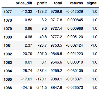
Here we calculate price_diff as difference between open price “today” and close price on the shifted target day column, multiply it by our stake and signal sign (latter determines if we guessed direction right or not).

Backtesting

In this paragraph I will use some classes I borrow here. You can find them in my repository, in this article I will show the usage. Here is the strategy class:

class MachineLearningForecastingStrategy(Strategy):   
    
    def __init__(self, symbol, bars, pred):
        self.symbol = symbol
        self.bars = bars

    def generate_signals(self):
        signals = pd.DataFrame(index=self.bars.index)
        signals['signal'] = pred
        return signals

Basically it just takes predictions from neural network and puts them into a Pandas column. After we create Portfolio class, where all the calculations are performed:

rfs = MachineLearningForecastingStrategy('LTC', test_set, pred)
signals = rfs.generate_signals()
portfolio = MarketIntradayPortfolio('LTC', test_set, signals, INIT_CAPITAL, STAKE)
returns = portfolio.backtest_portfolio()

It takes dataframe of the test set prices, signals, initial capital value and the amount we are risking on every traded (fixed for this tutorial).

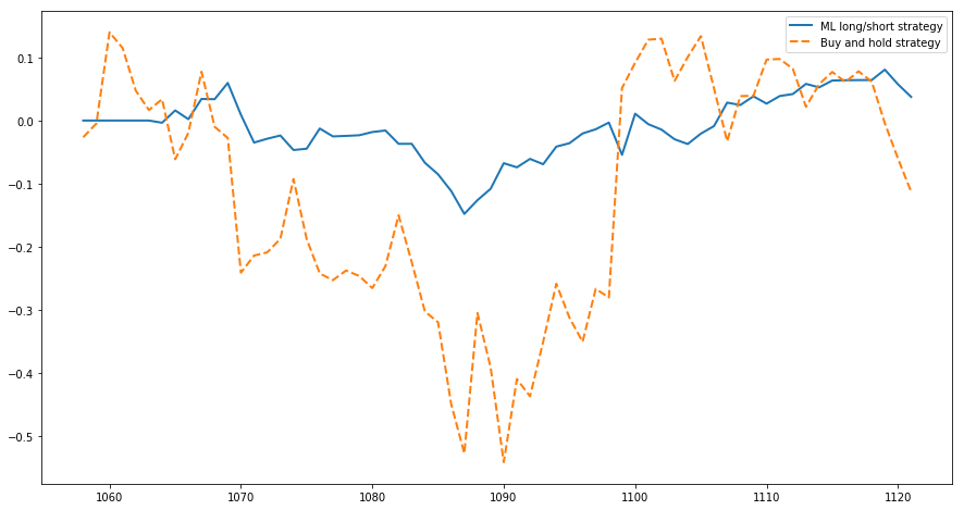
After running it we can plot the results on how our portfolio could develop with neural network signals versus of just holding the assets:

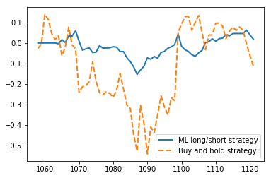
We can see, that our strategy has much less drawdown, is less volatile and ends up with a bit higher revenue — from 10000 to 10053 (which is basically nothing hehe). Sharpe ratios of these strategies are following: -3.04 for ML strategy and -4.68 for buy and hold — both are not cool at all, but let’s try all the process on another currency like ETH.

Neural network trained with following results:

MATTHEWS CORRELATION
0.07782916852651416
CONFUSION MATRIX
[[0.43333333 0.60714286]
 [0.33333333 0.64285714]]
CLASSIFICATION REPORT
             precision    recall  f1-score   support

          0       0.57      0.43      0.49        30
          1       0.51      0.64      0.57        28

avg / total       0.54      0.53      0.53        58

And backtesting shows following:

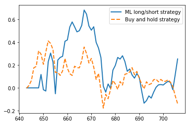
with Sharpe ratios of 6.90 and 7.57 respectively (even both strategies and up with losses in portfolio in this period).

Conclusion

We can learn following lessons from the results above:

Simple long/short strategies can be easily tested without any backtesting tools
Always compute confusion matrix, precision and recall of classifiers
Good forecasting accuracy (more than 55%) doesn’t mean high revenue of the strategy
Even simple “neural networks” with regularization can perform very well
Published by : Alexandr Honchar

The recent thought

Friday, March 16, 2018