K-Means & Other Clustering Algorithms: A Quick Intro with Python

     

   

 

Au     thor: Nikos Koufos

Author: Brendan Martin


K-Means & Other Clustering 

Algorithms:A Quick Intro with Python

Unsupervised learning via clustering algorithms. Let's work with the Karate Club dataset to perform several types of clustering algorithms.

Clustering is the grouping of objects together so that objects belonging in the same group (cluster) are more similar to each other than those in other groups (clusters). In this intro cluster analysis tutorial, we'll check out a few algorithms in Python so you can get a basic understanding of the fundamentals of clustering on a real dataset.

ARTICLE RESOURCES

• Source code: Github.
• Dataset: available via networkx library (see code below), also see paper: An Information Flow Model for Conflict and Fission in Small Groups

THE DATASET

For the clustering problem, we will use the famous Zachary’s Karate Club dataset. For more detailed information on the study see the linked paper.

Essentially there was a karate club that had an administrator “John A” and an instructor “Mr. Hi”, and a conflict arose between them which caused the students to split into two groups; one that followed John and one that followed Mr. Hi.

The students are the nodes in our graph, and the edges, or links, between the nodes are the result of social interactions outside of the club between students.

Since there was an eventual split into two groups (clusters) by the end of the karate club dispute, and we know which group each student ended up in, we can use the results as truth values for our clustering to gauge performance between different algorithms.

Social relationships (edges) of each student (node) outside of the Karate Club

GETTING STARTED WITH CLUSTERING IN PYTHON

Imports for this tutorial

from sklearn import cluster
import networkx as nx
from collections import defaultdict
import matplotlib.pyplot as plt
from matplotlib import cm
import seaborn as sns
import pandas as pd
import numpy as np
from sklearn.metrics.cluster import normalized_mutual_info_score
from sklearn.metrics.cluster import adjusted_rand_score
    

We'll be using the scikit-learn, pandas , and numpy stack with the addition of matplotlib, seaborn and networkx for graph visualization. A simple pip/conda install should work with each of these.

Let's go ahead and import the dataset directly from networkx and also set up the spring layout positioning for the graph visuals:

G = nx.karate_club_graph()

pos = nx.spring_layout(G)
    

Let's go ahead a create a function to let us visualize the dataset:

def draw_communities(G, membership, pos):
    """Draws the nodes to a plot with assigned colors for each individual cluster
    Parameters
    ----------
    G : networkx graph
    membership : list
        A list where the position is the student and the value at the position is the student club membership.
        E.g. `print(membership[8]) --> 1` means that student #8 is a member of club 1.
    pos : positioning as a networkx spring layout
        E.g. nx.spring_layout(G)
    """ 
    fig, ax = plt.subplots(figsize=(16,9))
    
    # Convert membership list to a dict where key=club, value=list of students in club
    club_dict = defaultdict(list)
    for student, club in enumerate(membership):
        club_dict[club].append(student)
    
    # Normalize number of clubs for choosing a color
    norm = colors.Normalize(vmin=0, vmax=len(club_dict.keys()))
    
    for club, members in club_dict.items():
        nx.draw_networkx_nodes(G, pos,
                               nodelist=members,
                               node_color=cm.jet(norm(club)),
                               node_size=500,
                               alpha=0.8,
                               ax=ax)

    # Draw edges (social connections) and show final plot
    plt.title("Zachary's Karate Club")
    nx.draw_networkx_edges(G, pos, alpha=0.5, ax=ax)
    

In order to color the student nodes according to their club membership, we're using matplotlib's Normalize class to fit the number of clubs into the (0, 1) interval. You might be wondering why we need to do this when there's only two clubs that resulted from the study, but we'll find out later that some clustering algorithms didn't get it right and we need to be able to colorize more than two clubs.

To compare our algorithm's, performance we want the true labels, i.e. where each student ended up after the club fission. Unfortunately, the true labels are not provided in the networkxdataset, but we can retrieve them from the study itself and hardcode them here:

# True labels of the group each student (node) unded up in. Found via the original paper
y_true = [0, 0, 0, 0, 0, 0, 0, 0, 1, 1, 0, 0, 0, 0, 1, 1, 0, 0, 1, 0, 1, 0, 1, 1, 1, 1, 1, 1, 1, 1, 1, 1, 1, 1]
    

Now, let's use our draw function to visualize the true student club membership and their social connections:

draw_communities(G, y_true, pos)
    

RESULT:

This is the true division of the Karate Club. We'll see how our algorithms do when trying to cluster on their own below.

Before that, we need to preprocess the data by transforming the graph into a matrix since that is the format required for the clusterers. Remember this edge_mat variable below, we'll be using this for input to our clustering models in the next few sections:

def graph_to_edge_matrix(G):
    """Convert a networkx graph into an edge matrix.
    See https://www.wikiwand.com/en/Incidence_matrix for a good explanation on edge matrices
   
    Parameters
    ----------
    G : networkx graph
    """
    # Initialize edge matrix with zeros
    edge_mat = np.zeros((len(G), len(G)), dtype=int)

    # Loop to set 0 or 1 (diagonal elements are set to 1)
    for node in G:
        for neighbor in G.neighbors(node):
            edge_mat[node][neighbor] = 1
        edge_mat[node][node] = 1

    return edge_mat
    

Let's transform our graph into a matrix and print the result to see what it contains:

edge_mat = graph_to_edge_matrix(G)
edge_mat

"""
array([[1, 1, 1, ..., 1, 0, 0],
       [1, 1, 1, ..., 0, 0, 0],
       [1, 1, 1, ..., 0, 1, 0],
       ..., 
       [1, 0, 0, ..., 1, 1, 1],
       [0, 0, 1, ..., 1, 1, 1],
       [0, 0, 0, ..., 1, 1, 1]])
"""
    

CLUSTERING ALGORITHMS

Unsupervised learning via clustering can work quite well in a lot of cases, but it can also perform terribly. We'll go through a few algorithms that are known to perform very well and see how the do on the same dataset. Fortunately, we can use the true cluster labels from the paper to calculate metrics and determine which is the best clustering option.

K-Means Clustering

 

N (the number of node):

K (the number of cluster):

Source: github.com/nitoyon/tech.nitoyon.com

K-means is considered by many to be the gold standard when it comes to clustering due to its simplicity and performance, so it's the first one we'll try out.

When you have no idea at all what algorithm to use, K-means is usually the first choice.

K-means works by defining spherical clusters that are separable in a way so that the mean value converges towards the cluster center. Because of this, K-Means may underperform sometimes.

To simply construct and train a K-means model, we can use sklearn's package. Before we do, we are going to define the number of clusters we know to be true (two), a list to hold results (labels), and a dictionary containing each algorithm we end up trying:

k_clusters = 2
results = []
algorithms = {}

algorithms['kmeans'] = cluster.KMeans(n_clusters=k_clusters, n_init=200)
    

To fit this model, we could simply call algorithms['kmeans'].fit(edge_mat).

Since we'll be testing a bunch of clustering packages, we can loop over each and fit them at the same time. See below.

Agglomerative Clustering

The main idea behind Agglomerative clustering is that each node first starts in its own cluster, and then pairs of clusters recursively merge together in a way that minimally increases a given linkage distance.

The main advantage of Agglomerative clustering (and hierarchical clustering in general) is that you don’t need to specify the number of clusters. That of course, comes with a price: performance. But, in sklearn’s implementation, you can specify the number of clusters to assist the algorithm’s performance.

You can find a lot more information about how this technique works mathematically here.

Let's create and train an agglomerative model and add it to our dictionary:

algorithms['agglom'] = cluster.AgglomerativeClustering(n_clusters=k_clusters, linkage="ward")
    

Spectral Clustering

The Spectral clustering technique applies clustering to a projection of the normalized Laplacian. When it comes to image clustering, Spectral clustering works quite well.

algorithms['spectral'] = cluster.SpectralClustering(n_clusters=k_clusters, affinity="precomputed", n_init=200)
    

Affinity Propagation

Affinity propagation is a bit different. Unlike the previous algorithms, this one does not require the number of clusters to be determined before running the algorithm.

Affinity propagation performs really well on several computer vision and biology problems, such as clustering pictures of human faces and identifying regulated transcripts, but we'll soon find out it doesn't work well for our dataset.

Let's add this final algorithm to our dictionary and wrap it all up by fitting each model:

algorithms['affinity'] = cluster.AffinityPropagation(damping=0.6)

# Fit all models
for model in algorithms.values():
    model.fit(edge_mat)
    results.append(list(model.labels_))
    

METRICS & PLOTTING

Well, it is time to choose which algorithm is more suitable for our data. A simple visualization of the result might work on small datasets, but imagine a graph with one thousand, or even ten thousand, nodes. That would be slightly chaotic for the human eye. So, let calculate the Adjusted Rand Score (ARS) and the Normalized Mutual Information (NMI) metrics for easier interpretation.

Normalized Mutual Information (NMI)

Mutual Information of two random variables is a measure of the mutual dependence between the two variables. Normalized Mutual Information is a normalization of the Mutual Information (MI) score to scale the results between 0 (no mutual information) and 1 (perfect correlation). In other words, 0 means dissimilar and 1 means
a perfect match.

Adjusted Rand Score (ARS)

Adjusted Rand Score on the other hand, computes a similarity measure between two clusters. ARS considers all pairs of samples and counts pairs that are assigned in the same or different clusters in the predicted and true clusters.

If that's a little weird to think about, have in mind that, for now, 0 is the lowest similarity and 1 is the highest.

In order to plot our scores, let's first calculate them. Remember that y_true is still a dictionary where the key is a student and the value is the club they ended up in. We need to get y_true's values first in order to compare them to y_pred:

nmi_results = []
ars_results = []

y_true_val = list(y_true.values()

# Append the results into lists
for y_pred in results:
    nmi_results.append(normalized_mutual_info_score(y_true_val, y_pred))
    ars_results.append(adjusted_rand_score(y_true_val, y_pred))
    

Let's now plot both scores side-by-side along with their averages for a better comparison.

We're using Seaborn's barplot along with matplotlib just for simpler coloring syntax. Most of the following is pretty simple.

The only thing fancy we added was the text on top of the bars. This is achieved on each subplot by referencing each axes (subplot), then using the index (i) as the x-coordinate, the score (v) as the y-coordinate, followed by the rounded value of v as the actual text to show on top.

fig, (ax1, ax2, ax3) = plt.subplots(1, 3, sharey=True, figsize=(16, 5))

x = np.arange(len(y))
avg = [sum(x) / 2 for x in zip(nmi_results, ars_results)]

xlabels = list(algorithms.keys())

sns.barplot(x, nmi_results, palette='Blues', ax=ax1)
sns.barplot(x, ars_results, palette='Reds', ax=ax2)
sns.barplot(x, avg, palette='Greens', ax=ax3)

ax1.set_ylabel('NMI Score')
ax2.set_ylabel('ARS Score')
ax3.set_ylabel('Average Score')

# # Add the xlabels to the chart
ax1.set_xticklabels(xlabels)
ax2.set_xticklabels(xlabels)
ax3.set_xticklabels(xlabels)

# Add the actual value on top of each bar
for i, v in enumerate(zip(nmi_results, ars_results, avg)):
    ax1.text(i - 0.1, v[0] + 0.01, str(round(v[0], 2)))
    ax2.text(i - 0.1, v[1] + 0.01, str(round(v[1], 2)))
    ax3.text(i - 0.1, v[2] + 0.01, str(round(v[2], 2)))

# Show the final plot
plt.show()
    

RESULT:

As you can see in the resulting chart, K-means and Agglomerative clustering have the best possible outcome for our dataset. That, of course, does not mean that Spectral and Agglomerative are low-performing algorithms, just that the did not fit in our particular dataset.

Out of curiosity, let's create a new function to plot where each algorithm went wrong by comparing the predicted student clusters with the true student clusters:

def draw_true_vs_pred(G, y_true, y_pred, pos, algo_name, ax):
    
    for student, club in y_true.items():
        if y_pred is not None:
            if club == y_pred[student]:
                node_color = [0, 1, 0]
                node_shape = 'o'
            else:
                node_color = [0, 0, 0]
                node_shape = 'X'
                
        nx.draw_networkx_nodes(G, pos,
                               nodelist=[student],
                               node_color=node_color,
                               node_size=250,
                               alpha=0.7,
                               ax=ax,
                               node_shape=node_shape)
    
    # Draw edges and show final plot
    ax.set_title(algo_name)
    nx.draw_networkx_edges(G, pos, alpha=0.5, ax=ax)


fig, ((ax1, ax2), (ax3, ax4)) = plt.subplots(2, 2, sharex=True, sharey=True, figsize=(10, 10))

for algo_name, ax in zip(algorithms.keys(), [ax1, ax2, ax3, ax4]):
    draw_true_vs_pred(G, y_true, algorithms[algo_name].labels_, pos, algo_name, ax)
    

RESULT:

This graph depicts each algorithm's correct (green circle) and incorrect (black X) cluster assignments.

Interestingly, we see that although the Affinity algorithm had a higher average score, it only put one node in the correct cluster.

To see the reason why, we can look at the cluster information from that algorithm:

cluster_centers_indices = algorithms['affinity'].cluster_centers_indices_
n_clusters_ = len(cluster_centers_indices)
print(n_clusters_)
# 8
    

Since we were not able to define the number of clusters for Affinity Propagation, it determined that there were eight clusters. Our metrics didn't hint at this problem since our scoring wasn't based off of clustering accuracy.

Let's wrap it up but taking a look at what our Affinity algorithm actually clustered:

# The resulting clubs
algorithms['affinity'].labels_

# array([0, 2, 2, 2, 1, 1, 1, 2, 4, 3, 1, 1, 2, 2, 4, 4, 1, 2, 4, 4, 4, 2, 4, 5, 5, 6, 3, 3, 6, 4, 5, 7, 7], dtype=int64)

draw_communities(G, algorithms['affinity'].labels_, pos)
    

RESULT:

FINAL WORDS

Thanks for joining us in this clustering introduction. I hope you found some value in seeing how we can easily manipulate a public dataset and apply and compare several different clustering algorithms using sklearn in Python.

If you have any questions, definitely let us know in the comments below. Also, feel free to attach a clustering project you've experimented with!

Quantum Machine Learning 1.0 A big future for small devices

Quantum Machine Learning 1.0

A big future for small devices

Quantum machine learning is a new buzzword in quantum computing. This emerging field asks — amongst other things — how we can use quantum computers for intelligent data analysis. At Xanadu we are very excited about quantum machine learning and spend a fair amount of time thinking about it. Here is why.

First of all, it is important to note that quantum machine learning is very young, meaning that it is not yet clear what results, and commercial applications, to expect from it. This was demonstrated at the “Quantum meets Industry” panel at the quantum machine learning conference in Bilbao, Spain. When asked whether the time is ripe for commercial investments into quantum machine learning, the experts from companies such as IBM, Microsoft and NASA, were noticeably careful with their answers. Still, almost every company involved in quantum computing today, including the representatives in the panel, has a machine learning group.

If even the ‘big players’ are struggling to make definite statements about the — let’s say 5-year — outlook on using quantum computers for machine learning tasks, should quantum computing startups like Xanadu get on board? We think the answer is yes and want to put three arguments forward:

1. Early-generation quantum devices are promising newcomers to the growing collection of AI accelerators, thereby enabling machine learning.
2. Quantum machine learning can lead to the discovery of new models and thereby innovate machine learning.
3. Machine learning, and quantum machine learning in particular, will increasingly permeate all aspects of quantum computing, redefining the way we think about quantum computing.

Let us go through these points one by one.

1. Enable machine learning

Early-generation quantum devices vary in their programming models, their generality, the quantum advantage they promise, and the hardware platforms that they run on. Across the board, they are very different from the universal processors that researchers envisioned when the field started in the 1990s. For machine learning, this may be a feature rather than a bug.

Quantum devices as special-purpose AI accelerators

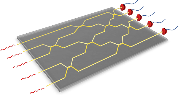
An example of a “quantum ASIC” is an integrated nanophotonics chip that implements Boson sampling for a fixed number of modes (here corresponding to yellow light beams). Boson sampling quickly becomes intractable on classical computers if we increase the number of modes.

Many current quantum technologies resemble special-purpose hardware like Application-Specific Integrated Circuits (ASICs), rather than a general-purpose CPU. They are hardwired to implement a limited class of quantum algorithms. More advanced quantum devices can be programmed to run simple quantum circuits, which makes them more similar to Field-Programmable Gate Arrays (FPGAs), integrated circuits that are programmed using a low-level, hardware-specific Hardware Description Language. In both cases, an intimate knowledge of the hardware design and limitations is needed to run effective algorithms.

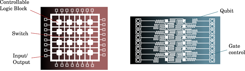
Schematic drawing of an FPGA (left) and IBM’s 16 qubit quantum chip (right, adapted from here). Near-term quantum devices can be compared to FPGAs, in that they also consist of locally programmable gates with a hardware-oriented programming language.

ASICs and FPGAs find growing use in machine learning and artificial intelligence, where their slim architectures reduce the overhead of a central processor and naturally suit the task they specialize in. If current quantum technologies resemble this classical special-purpose hardware, they could find applications in machine learning in a similar fashion. And this even without universal quantum computing and exponential quantum speedups.

“Quantum technologies may eventually have a place in the mix of AI hardware as we develop newer and newer techniques to advance towards artificial general intelligence.”

Taking a look at the most advanced AI solutions reveals that they already use a blend of technologies. More and more computation is done on special-purpose devices located at the edge, where technology interacts with its environment (think of fingerprint recognition for unlocking a phone or smile detection in a camera). At the other end of the spectrum, calculations are done on GPU clusters (for instance, traffic routing or tagging photos). As a matter of fact, a modern GPU is already a technology blend in itself: the latest Volta chips by Nvidia include low-precision ASICs called Tensor Cores, designed specifically to accelerate the training of neural networks. Google follows a similar path with their Tensor Processing Units (TPUs) that are designed to support the TensorFlow machine learning framework. In short, AI has already embraced heterogeneity. Quantum technologies may eventually have a place in the mix of AI hardware. And this mix has to be as strong as possible if we want to advance towards artificial general intelligence.

Finally, hardware can significantly shape the advancement of software. In the 2010s, the use of GPUs contributed to the renaissance of neural network models (that have been around for decades but were largely discarded as untrainable). Similarly, accelerating quantum technologies could make their very own contribution to lifting specific machine learning methods into the realm of the doable, or even of the cutting-edge. This is particularly true for methods that are considered too hard to train with classical hardware and which were superseded by more convenient competitors.

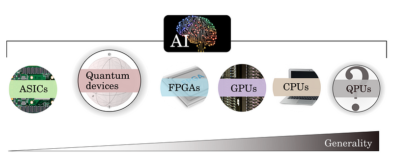
Future artificial intelligence and machine learning applications will need multiple hardware platforms, where every component is responsible for certain subtasks. Early-generation quantum devices could find their place on the low-generality (but high-speed) end of AI accelerators. One day, an error-corrected general purpose quantum processing unit (QPU) could extend the spectrum towards the right.

What quantum computers are good at

If early-generation quantum devices can be thought of as special-purpose AI accelerators, what exactly can quantum computers contribute to machine learning and AI? Why would we want to use “quantum ASICs”? Let’s look at a selection of exciting candidate tasks, namely optimization, linear algebra, sampling, and kernel evaluations.

Optimization. Just like in machine learning, optimization is a prominent task in quantum physics. Physicists (and quantum chemists) are typically interested in finding the point of lowest energy in a high-dimensional energy landscape. This is the basic paradigm of adiabatic quantum computing and quantum annealing. To no surprise, one of the first tasks for quantum computers investigated in the context of machine learning was optimization. The D-Wave quantum annealer, a special-purpose device that can solve so-called quadratic unconstrained binary optimization problems, was used as early as 2008 to solve classification tasks. More recently, the hybrid quantum-classical technique of variational circuits has been proposed. There, a quantum device is used to evaluate a hard-to-compute cost function, while a classical device performs an optimization based on this information.

Linear Algebra. When speaking about potential exponential quantum speedups for machine learning, people usually refer to the inherent ability of quantum computers for executing linear algebra computations. There are many subtleties to this claim, and its prospect with regards to hardware in the near term is not always clear. One of the bottlenecks is data encoding: to use a quantum computer as a kind of super-fast linear algebra enabler for large matrix multiplications and eigendecompositions (not unlike TPUs), we have to first “load” the large matrix onto the quantum device, a procedure that is highly non-trivial.

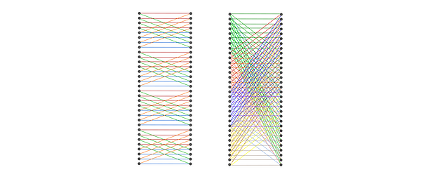
If we interpret the matrix describing a quantum gate as a linear layer of a neural network, we can visualize how the gate would connect inputs and outputs (which are ultimately the amplitudes of the quantum state). A single qubit gate can transform an exponentially large vector, yet in a highly symmetric fashion. Left: Arbitrary single qubit gate applied to the third out of five qubits. Right: Arbitrary two qubit gate applied to the third and fourth out of five qubits. Each shade of a color stands for a different “weight”.

However, there may be near-term benefits in understanding quantum computers as fast linear algebra processing units. Mathematically speaking, a quantum gate executes a multiplication of an exponentially — or even infinitely — large matrix with a similarly large vector. Specific costly linear algebra computations — namely those corresponding to quantum gates — can be therefore be done in a single operation on a quantum computer. This perspective is leveraged when building machine learning models out of quantum algorithms, for example when we think of an quantum gate as a (highly structured) linear layer of an enormous neural network.

Sampling. All quantum computers can be understood as samplers that prepare a special class of distributions (quantum states) and that sample from these distributions via measurements. A very promising avenue is therefore to explore how samples from quantum devices can be used to train machine learning models. This has been investigated for Boltzmann machines and Markov logic networks, where the so called Gibbs distribution — which is inspired by physics and hence comparably easy to realize with a physical system — plays an important role.

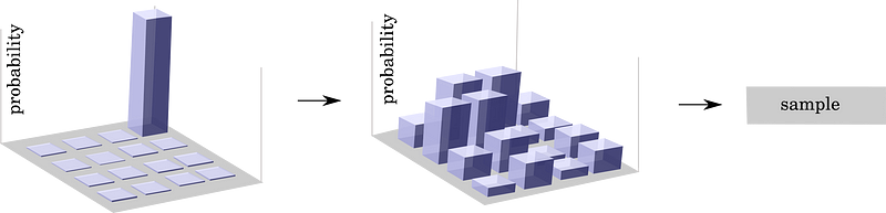
Every quantum computer is fundamentally a sampler that starts with a simple probability distribution over all possible measurement outcomes, computes a more complicated distribution, and samples an outcome via a measurement. Quantum devices are therefore interesting assistants for sampling-based training, for example with Boltzmann machines.

“We should think of early-generation quantum computers as small, partially programmable special-purpose devices that can take over costly jobs for machine learning which naturally suit them.”

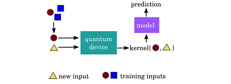
Kernel evaluation. One very recent idea from Xanadu illustrates how there are more specific tasks in machine learning that could be taken over by quantum devices. Kernel methods use machine learning models based on a distance measure between data points which is called a kernel. Quantum devices can be used to estimate certain kernels, including ones that are difficult to compute classically. The estimates from the quantum computer can be fed into a standard kernel method — such as a support vector machine. Inference and training are done purely classically, but augmented with the quantum special purpose device.

The idea of “quantum kernels” is to use the quantum device only to compute kernels of data points, by estimating the inner product of two very high-dimensional quantum states. The kernel estimates can then be fed into a classical machine learning model for training and prediction. 

In summary, we should think of early-generation quantum computers as small, partially programmable special-purpose devices that can accelerate certain tasks in machine learning, just like the way GPUs enabled deep learning.

2. Innovate machine learning

Besides enabling pre-existing machine learning techniques, quantum machine learning potentially has a lot more to offer. Recently, a growing number of physicists trained in the methods of quantum theory and quantum computing have begun to think about machine learning. Having physicists enter machine learning has proven fruitful in the past — just think of the physicist John Hopfield who introduced his intimate knowledge of the Ising model into machine learning and created what is now known as associative memory in Hopfield networks. Quantum computing can lead to entirely new machine learning models. These new models are tailor-made for quantum devices, and may turn out to be something that works well, but which the machine learning community has simply never thought up. Let us demonstrate this with two examples that are actively investigated in quantum machine learning.

Sampling from quantum distributions

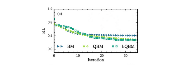
Results from Amin et al. (2018) showing the KL-divergence between the target and model distribution of a classical Boltzmann machine (BM) and two versions of a quantum Boltzmann machine (bQBM and QBM) during training. After a few iterations, both quantum models show better results than classical model. [Figure has been slightly adapted.]

It was mentioned above that quantum devices are good at sampling. For example, quantum annealers can be used to approximately sample from a Gibbs distribution to train Boltzmann machines. But this is not straightforward, since the quantum device actually prepares a quantum Gibbs distribution. Instead of trying to “make things classical”, researchers investigated what happens if we use the natural quantum distribution. It turns out that in some cases, “quantum samples” can be very useful for training, as shown in the figure on the left.

“Discovering new machine learning models is similar to searching for gold on a yet unknown island. In the case of quantum machine learning, we have found some promising signs of gold at the first beach, which is why we are building better expedition gear and venturing further — excited by what we might find.”

Variational quantum circuits

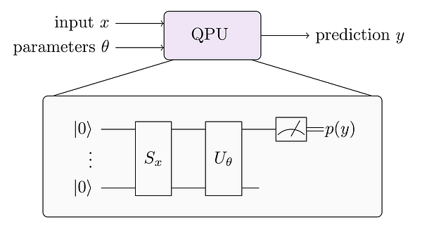
As a second example, consider a programmable quantum device — where “programmable” refers to some device parameters that can be tuned to change the specifications of an otherwise fixed computation. We set some of these parameters to the values of input data x, and associate other parameters as trainable variables θ. The device ultimately gives us some outputs y = f(x, θ) that depend on inputs and variables. Such a quantum device (and this description is really very generic) implements a supervised learning model. This model is sometimes called a variational classifier, relating it to the concept of variational (i.e., trainable) quantum circuits. In a similar way we can construct unsupervised models.

A programmable quantum device can be interpreted as a supervised machine learning model that computes y=f(x, θ). The trainable parameters θ can be learned via classical optimization. The figure is taken from this paper.

The function f that the quantum device computes can be very specific to its hardware architecture, how parameters enter the computation, and how one relates variables, inputs, and outputs to the quantum algorithm. However, altogether we get a “quantum model”. Importantly, if we do not know how to simulate the quantum model with a classical computer, we have not only a new ansatz to do machine learning, but also one that can only be executed with a quantum device. The emerging literature on variational circuits shows how to train such “hardware-derived” models with classical computers, and groups around the world are currently busy investigating the power and limits of such quantum models.

Discovering new machine learning models is similar to searching for gold on a yet unknown island. In the case of quantum machine learning, we have found some promising signs of gold at the first beach, which is why we are building better expedition gear and venturing further — excited by what we might find.

3. Redefine the way we think about quantum computing

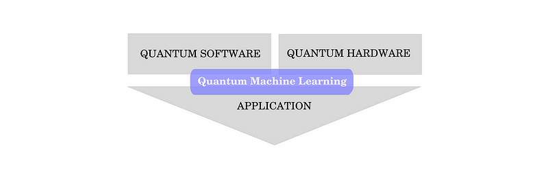
There is a third, more “behind-the-scenes” reason why we think that quantum machine learning is essential. Quantum machine learning, and its central subtask, optimization, are not only subfields of quantum computing, they are increasingly becoming approaches to quantum computing itself. As such, they have the potential to redefine the way we think about quantum computing. This holds for software design, hardware development and applications that rely on quantum computing.

Quantum machine learning is not only a potential application for quantum computing, but a way of thinking that permeates all of its aspects.

Quantum software design

So far, quantum algorithms are carefully composed by people who have a deep knowledge of the tricks of the trade. And even the “bible” of quantum computing, the textbook of Michael Nielsen and Isaac Chuang, remarks that “coming up with good quantum algorithms seems to be a difficult problem”. But quantum algorithms could also be learned.

Consider for example the preparation of resource states. Resource states feature widely, i.e., in continuous-variable applications or error correction with magic states, where the computation relies on a specific state to be prepared as an input. Oftentimes, the algorithm to prepare the initial state is unknown. However, given a device with a certain type of gates, we can let the computer “learn” a gate sequence that prepares the desired state on the specific hardware. Likewise, entire quantum experimental setups (i.e., to generate highly entangled quantum systems) have been designed by machine learning approaches.

“The ideas of machine learning can transform the way we do quantum algorithmic design: Instead of composing algorithms, we can let the device learn them.”

Quantum hardware development

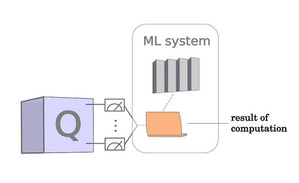
Machine learning is becoming increasingly popular for the post-processing of measurements in quantum computing. One day, the result of any quantum computation may rely on machine learning methods.

Intimate knowledge of machine learning can also help to build a quantum computer. Building a quantum computer will generate large amounts of labeled and unlabeled data. For example, data is generated when reading out the final quantum state of the device, when assessing the performance of gates, or when it comes to estimating measurement results. Quantum machine learning has a very active subfield, in which classical machine learning is used as a method to make sense of data produced by quantum experiments in the lab. Machine learning systems could easily become a standard component of quantum hardware.

“Machine learning may one day be a standard technique to read out the results of a computation with a quantum device.”

Applications

Quantum machine learning techniques are also closely tied with a variety of application areas. Quantum chemistry, for instance, is likewise interested in minimizing high-dimensional and difficult cost functions, e.g., to find the lowest energy configurations of molecules for drug discovery or material science. Quantum computers can be used to tackle these problems, with methods like the variational quantum eigensolvers mentioned above (see for example this recent result which scaled to a water molecule on an extremely noisy quantum computer).

Since machine learning and quantum chemistry are both heavily based on optimization, it is not surprising that they can both leverage similar quantum algorithms. A variational quantum eigensolver is, in essence, the same algorithm as a variational classifier, which was introduced as an innovative way to use quantum computers for machine learning. Understanding gained from the machine learning side will translate to new insights on the chemistry side. Good quantum machine learning algorithms will therefore have immediate consequences for other quantum applications based on data and optimization.

In summary, the potential of quantum machine learning to enable and innovate future AI applications, as well as to contribute towards the development of the field of quantum computing itself are three reasons why quantum machine learning may have a big future when it comes to small-scale quantum devices.

This opinion piece is signed by: Maria Schuld, Nathan Killoran, Thomas Bromley, Christian Weedbrook, Peter Wittek