Reinforcement Learning to solve Rubik’s cube (and other complex problems!)

Published By:Max Lapan

Foreword

Half a year has passed since my book “Deep Reinforcement Learning Hands-On” has seen the light. It took me almost a year to write the book and after some time of rest from writing I’ve discovered that explaining RL methods and turning theoretical papers into working code is a lot of fun for me and I don’t want to stop. Luckily, RL domain is evolving, so, there are lots of topics to write about.

Introduction

In mass perception, Deep Reinforcement Learning is a tool to be used mostly for game playing. This is not surprising, given the fact, that historically, the first success in the field was achieved in Atari game suite by Deep Mind in 2015.

Atari benchmark suite turned out to be very successful for RL problems and, even now, lots of research papers are using it for demonstrating the efficiency of their methods. As the RL field progresses, the classical 53 Atari games continue to become less and less challenging (at the time of writing more than half of games are solved with super-human accuracy) and researches turn to more complex games, like StarCraft and Dota2.

But this bias towards games creates a false impression “RL is about playing games’’, which is very far from the truth. In my book, published in June 2018,
I’ve tried to counterbalance this by accompanying Atari games with the examples from other domains, including stock trading (chapter 8), chatbots and NLP problems (chapter 12), web navigation automation (chapter 13), continuous control (chapters 14…16) and boards games (chapter 18).

In fact RL having very flexible MDP model potentially could be applied to a wide variety of domains, where computer games is just one convenient and spectacular example of the complicated decision making.

In this article I’ve tried to write a detailed description of the recent attempt to apply RL to a field of combinatorial optimisation. The paper discussed was published by the group of researchers from UCI (University of California, Irvine) and called “Solving the Rubik’s Cube Without Human Knowledge’’. In addition to the detailed description of the paper, we’ll cover my open-source PyTorch implementation of the method proposed, do experiments with training models and outline directions to improve the method proposed in the paper.

In the text below, I’ll interwine the description of the paper’s method with code pieces from my version to illustrate the concepts with the concrete implementation. If you’re interested only in the theoretical description of the method, you could easily skip the code.

Let’s start with the overview of Rubik’s cube and Combinatorial Optimisation in general.

Rubik’s cube and combinatorial optimisation

I doubt it’s possible to find a person who hasn’t heard about the Rubik’s Cube, so, I’m not going to repeat the Wikipedia description of this puzzle, but rather focus on connections it has to mathematics and computer science. If it’s not explicitly stated, by “cube’’ I mean 3x3 classical Rubik’s cube. There are lots of variations based on the original 3x3 puzzle, but they are still far less popular than the classical invention.

Being quite simple in terms of mechanic and task description, Rubik’s cube 3x3 is quite a tricky object in terms of all transformations we can make by possible rotations of the cube’s sides. It was calculated that in total, cube 3x3 has 4.33 × 10¹⁹ distinct states reachable by rotating the cube. That’s only the states which are reachable without disassembling the cube, by making thing apart and then assembling it, you can reach twelve times more states in total (≈5.19 × 10²⁰), but those “extra’’ states make cube unsolvable without disassembling.

All those states are quite intimately intertwined with each other by using rotations of the cube’s sides. For example, if we rotate the left side clockwise in some state, we get to the state, from which rotation of the same side counter-clockwise will destroy the effect of transformation and we’ll get into the original state. But if we apply the left side rotation three times in a row, the shortest path to the original state will be just a single rotation of the left side clockwise, but not three times counter-clockwise (which is also possible, just not optimal).

As cube 3x3 has 6 edges and each edge could be rotated in two directions, we have 12 possible rotations in total. Sometimes, half-turns (which are two consecutive rotations in the same direction) are also included as distinct rotations, but for simplicity, we’ll treat them as two distinct transformations of the cube.

In mathematics, there are several areas which study objects of this kind. First of all, it is “abstract algebra’’, very broad division of math, which studies abstract sets of objects with operations on top of them. In its terms, Rubik’s cube is an example of quite complicated group with lots of interesting properties.

But cube is not only states and transformations, it’s a puzzle, with primary goal is to find a sequence of rotations with solved cube in the end. Problems of this kind are studied by Combinatorial Optimisation, which is a sub-field of applied mathematics and theoretical computer science. This discipline has lots of famous problems of high practical value, to name a few:

• Travelling Salesman Problem: find the shortest closed path in a graph,
• Protein Folding Simulation: find possible 3D structures of protein,
• Resource Allocation: how to spread fixed set of resources among consumers to get the best objective,

and lots of others…

What those problems have in common is huge state space, which makes it infeasible to just check all possible combinations to find the best solution. And our “toy cube problem’’ also falls into the same category, because states space of 4.33 × 10¹⁹ makes brute force approach totally impractical.

Optimality and God’s number

What makes combinatorial optimisation problem tricky is that we’re not looking for any solution, we’re in fact interested in optimal solution of the problem. The difference is obvious: right after Rubik’s cube was invented, it is known how to reach the goal state (but it took Ernő Rubik about a month, to figure out the first method of solving his own invention, which, I guess, was rough experience). Nowadays, there are lots of different ways or “schemes’’ of cube solving: beginner’s method, method by Jessica Fridrich (very popular among speedcubers) and lots of others.

All of them vary by amount of moves to be taken. For example, a very simple beginner’s method requires about 100 rotations to solve the cube using 5…7 sequences of rotations to be memorized. In contrast, the current world record on speedcubing competition is to solve 3x3 cube in 4.22 seconds, which requires much less steps, but more sequences to be memorized and trained. The method by Jessica Fridrich requires about 55 moves in average, but you need to familiarize yourself with ≈120 different sequences of moves.

But, of course, the big question was: what is the shortest sequence of actions to solve any given state of the cube? Surprisingly, after 54 years of huge popularity of cube, humanity still doesn’t know the full answer to this question. Only in 2010, the group of researchers from Google has proven that the minimum amount of moves needed to solve any cube state is 20. This number is also known as God’s number. Of course, in average, the optimal solution is shorter, as only a bunch of states requires 20 moves and one single state doesn’t require any moves at all (solved state).

This result only proves the minimal amount of moves, but does not find the solution itself. How to find the optimal solution for any given state is still an open question.

Approaches to cube solving

Before the paper has been published, there were two major directions to solve Rubik’s cube:

1. by using the group theory results, it is possible to significantly reduce the state space to be checked. One of the most popular solver using this approach is Kociemba's algorithm,
2. by using the brute force search accompanied by manually-crafter heuristics to direct the search into the most promising direction. The vivid example of this is Korth's algorithm, which uses A* search with large database of patters to cut bad directions.

The paper has introduced the third approach: by training the neural network on lots of randomly shuffled cubes, it is possible to get the policy which will show us the direction towards the solved state. The training is done without any prior knowledge about the domain, the only thing needed is the cube itself (not the physical one, but the computer model of it). This is a contrast with the above two methods, which require lots of human knowledge about the domain and labour to implement them in a form of a computer code.

In the subsequent sections we’ll take a detailed look at this new approach.

Data representation

In the beginning, let’s start with data representation. In the 3x3 cube problem we have two entities to be encoded somehow: actions and states.

Actions

Actions are possible rotations we can do from any given cube state and as it has already been mentioned we have only 12 actions in total. There is established naming of actions followed from cube sides we’re rotating. Names of cube sides are left, right, top, bottom, front and back. For every side, we have two different actions, corresponding to clockwise and counter-clockwise rotation of the side (90° or –90°). One small, but very important detail is that
rotation is performed from position when the desired side is faced towards you. This is obvious for front side, for example, but for back side it might be confusing.

Names of actions are derived from the first letters of side’s name. For instance, rotation of the right side clockwise is named as R. There are different notations for counter-clockwise actions, sometimes they are denoted with apostrophe (R’) or with lower-case letter (r), or even with tilde (r̃). The first and the last notations are not very practical for computer code, so, in my implementation I’ve used lower case actions to denote counter-clockwise rotation. So, for the right side we have two actions: R and r, another two for the left side: L and l, and so on.

In my code, action space is implemented using python enum, where each action is mapped into the unique integer value.

States

A state is a particular configuration of cube stickers and as we have already mentioned, the size of our state space is very large (4.33 × 10¹⁹ different states). But the amount of states is not the only complication we have. In addition, we have different objectives we’d like to meet when we choose a particular representation of state:

• avoid redundancy: In the extreme, we can represent state of the cube by just recording colours of every sticker on every side. But if we just count the amount of such combinations, we get 6⁶*⁸= 6⁴⁸ ≈ 2.25 × 10³⁷, which is significantly larger than our cube’s state space size, which just means that this representation is highly redundant, for example, it allows all sides of the cube to have one single colour (except the centre cubelets). If you’re curious how we’ve got 6⁶*⁸, this is simple: we have 6 sides of cube, each having 8 small cubes (we’re not counting centres), so we have 48 stickers in total and each of them could be coloured in one of 6 colours.
• memory-efficiency: As we’ll see shortly, during the training and, even more, during the model application, we’ll need to keep in memory the large amount of different states of the cube, which might influence the performance of the process. So, we’d like the representation to be as compact as possible.
• performance of transformations: On the other hand, we need to implement all the actions applied to the state and those actions need to be done quickly. If our representation is very compact in terms of memory (uses bit-encoding, for example), but requires us to do a lengthy unpack process for every rotation of the cube’s side, our training will become too slow.
• neural-network friendliness: Not every data representation is equally good as an input for the neural network. This is true not only for our case, but for Machine Learning in general, for example in NLP it is common to use bag of words or word embeddings, in CV images are decoded from jpeg into raw pixels, Random Forests require data to be heavily feature-engineered and so on.

In the paper, every state of the cube is represented as 20 × 24 tensor with one-hot encoding. To understand how it’s done and why it has this shape, let’s start with the picture taken from the paper.

Stickers we need to track in the cube are marked with white

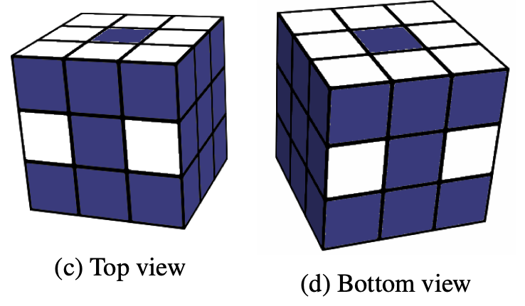
Here, with white colour we’ve marked the stickers of cubelets we need to track, the rest of stickers (coloured with blue) are redundant and there is no need to track them. As you know, 3x3 cube consists from three types of cubelets: 8 corner cubelets with three stickers, 12 side cubelets with two stickers and 6 central ones with a single sticker on it.

It might be not obvious from the first sight, but the central cubelets not needed to be tracked at all, as they cannot change their relative position and could only rotate. So, in terms of the central cubelets, we need only to agree on cube alignment and stick to it. For example, in my implementation white side is always on the top, front is red, left is green and so on. This makes our state rotation-invariant, which basically means, that all possible rotations of the cube as a whole are considered as the same state.

Ok, the central cubelets not tracked at all, that’s why on the figure on top all of them are marked with blue. What about the rest? Obviously, every cubelet of particular kind (corner or side) has its unique colour combination of the stickers. For example, the assembled cube in my orientation (white on top, red is front, etc) has top-left cubelet facing to us the following colours: green, white and red. There are no other corner cubelets with those colours (please check in case of doubt). The same is true for the side cubelets.

Due to this, to find position of some particular cubelet, we need to know the position of only one of its stickers. The selection of such stickers is completely arbitrary, but once selected, you need to stick to this. As shown on the figure above, we track eight stickers from the top side, eight stickers from the bottom and four additional side stickers, two on the front face and two on the backward. This gives us in total 20 stickers to be tracked.

Now, where “24'’ in tensor dimension comes from. In total we have 20 different stickers to track, but in which positions could they appear due to cube transformations? It depends on the kind of cubelet we’re tracking. Let’s start with corner cubelets. In total there are 8 of corner cubelets and cube transformations can reshuffle them in any order. So, any particular cubelet could end up in any of 8 possible corners. In addition, every corner cubelet could be rotated, so, our “green white red” cubelet could end up in three possible orientations:

• white on top, green left and red front,
• green on top, red left and white front,
• red on top, white left and green front.

So, to precisely indicate the position and the orientation of the corner cubelet, we have 8×3=24 different combinations.

In case of 12 side cubelets, they have only two stickers, so only two orientations possible, which again, gives us 24 combinations, but they are
obtained from different calculation: 12×2=24. And, finally, we have 20 cubelets to be tracked, 8 corner and 12 side, each having 24 positions
it could end up.

The very popular option to feed such data into neural networks is one-hot encoding, when the concrete position of the object has 1 with other positions
are filled with zero. This gives us the final representation of state as tensor with shape 20×24.

From redundancy point of view, this representation is much closer to the total state space, the amount of possible combinations equals to 24²⁰ ≈ 4.02 × 10²⁷. It is still larger than cube state space (it could be said it is significantlylarger, factor of 10⁸ is a lot), but it is better than encoding of all colours of every sticker. This redundancy comes from tricky properties of cube transformations, for example, it is not possible to rotate one single corner cubelet (or flip one side cubelet) leaving all others on their places.

Mathematical properties are well beyond of the scope of this article, if you’re interested, I could recommend the wonderful book by Alexander Frey and David Singmaster “Handbook of Cubic Math’’.

Careful readers might notice that tensor representation of cube state has one significant drawback: memory inefficiency. Indeed, by keeping state as
floating-point tensor of 20 × 24, we’re wasting 4 × 20 × 24 = 1920 bytes of memory, which is a lot, given the requirement to keep around thousands of states during the training process and millions of them during the cube solving (as you’ll get to know shortly). To overcome this, in my implementation, I’m using two representations: tensor one is intended for neural network input and another, much more compact representation is needed to store different states for longer. This compact state is saved as a bunch of lists, encoding permutations of corner and side cubelets and their orientation. This representation is not only much more memory efficient (160 bytes) but also much more convenient for transformations implementation.

The concrete details could be found in this module, the compact state is implemented in State namedtuple and the neural network representation is produced by function encode_inplace.

Training process

Now we know how the state of the cube is encoded in 20 × 24 tensor, let’s talk about the Neural Network architecture and how it is trained.

NN architecture

On the figure (taken from the paper), the network architecture is shown.

As the input it accepts the already familiar cube state representation as
20 × 24 tensor and produces two outputs:

• policy, which is a vector of 12 numbers, representing probability distribution over our actions,
• value, single scalar estimating the “goodness’’ of the state passed. The concrete meaning of a value will be discussed later.

Between input and output, network has several fully-connected layers with ELU activations. In my implementation, architecture is exactly the same as in the paper and could be found here.

Training

The network is quite simple and straightforward: policy says us what transformation we should apply to the state, the value estimates how good the state is. But the big question still remains: how to train the network?

The training method proposed in the paper has the name “Auto-Didactic Iterations’’ or ADI for short and it has surprisingly simple structure. We start with the goal state (the assembled cube) and apply the sequence of random transformations of some pre-defined length N. This gives us sequence of Nstates. For each state s in this sequence we do the following procedure:

• apply every possible transformations (12 in total) to the state s,
• pass those 12 states to our current neural network, asking for valueoutput. This gives us 12 values for every sub-state of s.
• target value for state s is calculated as vᵢ = maxₐ(v(sᵢ,a)+R(A(sᵢ,a))), where A(s, a) is the state after action a applied to the state s and R(s)equals 1 if s is the goal state and -1 otherwise.
• target policy for state s is calculated using the same formula, but instead of max we take argmax: pᵢ = argmaxₐ (v(sᵢ,a)+R(A(sᵢ,a))). This just means that our target policy will have 1 at the position of maximum value for sub-state and 0 on all other positions.

This process is shown on figure taken from the paper. The sequence of scrambles x₀, x₁… is generated, where cube xᵢ is shown expanded. For this state xᵢ, we make targets for the policy and value heads from the expanded states by applying the formulas above.

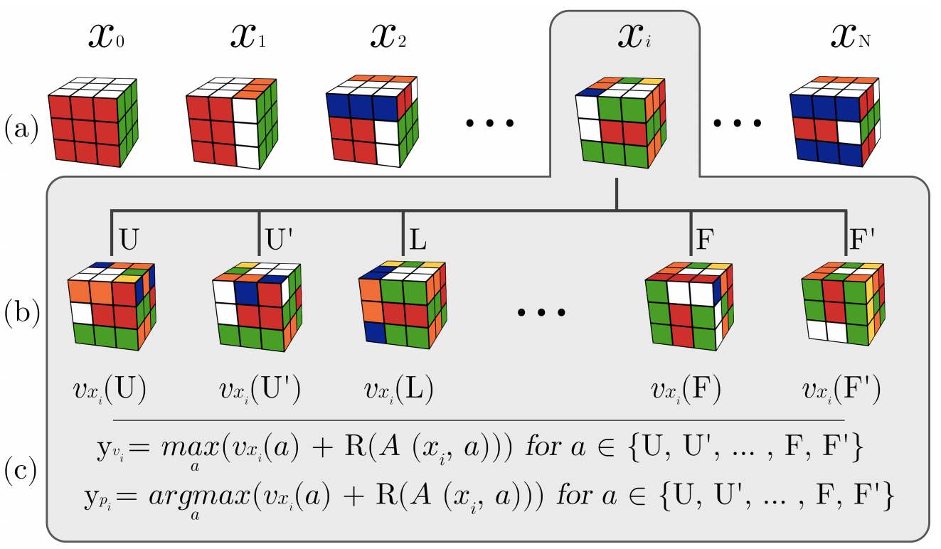
Using this process, we can generate any amounts of training data we want.

Model application

Ok, imagine we have trained the model using the process just described. How we should use it to solve scrambled cube? From the network structure, you might imagine the obvious (but, unfortunately, not very successful) way:

1. feed the model the current state of the cube we want to solve,
2. from the policy head get the largest action to perform (or sample it from resulting distribution),
3. apply the action to the cube,
4. repeat the process until the solved state has been reached.

Intuitively, this method should work, but in practice, it has one serious issue: it doesn’t. The main reason for that is our model quality. Due to the size of the state space and the nature of the neural networks, it is just not possible to train NN to return the exact optimal action for any input state all of the time. Rather than telling us what to do to get the solved state, our model shows us the promising directions to explore. Those directions could bring us closer to the solution, but sometimes they could be misleading, just from the fact that this particular state has never been seen during the training (don’t forget, there are 4.33 × 10¹⁹ of them, even with GPU’s training speed of hundreds of
thousands states per second, after a month of training we’ve got the chance to see the tiny portion of the state space, something about 0.0000005%. So, the more sophisticated approach has to be used.

And there is a family of very popular methods, called “Monte-Carlo Tree Search’’ or MCTS for short. There are lots of variants of those methods,
but the overall idea is simple and could be described in comparison to the well-known brute-force search methods, like “Breadth-First Search’’ (BFS) or
“Depth-First Search’’ (DFS). In BFS and DFS we perform the exhaustive search of our state space by trying all the possible actions and exploring all the states we get by those actions. As you can see, that behaviour is the another extreme of the procedure described above (when we have something which tells us where to go at every state).

MCTS offers something in between of those extremes: we want to perform the search and we have some information where we should go, but this information could be unreliable, noisy or just wrong at some situations. But sometimes, this information could show us the promising directions which could speed up the search process.

As I’ve mentioned, MCTS is a family of methods, which vary in particular details and characteristics. In the paper, the method called UCT (Upper Confidence bound1 applied to Trees) is used. The method operates on the tree, where the nodes are the states and the edges are actions, connecting those states. The whole tree is enormous in most of the cases, so, we not trying to build the whole tree, just some tiny portion of it. In the beginning, we start with a tree consisting of the single node, which is our current state.

On every step of the MCTS, we’re walking down the tree exploring some path in the tree, and there are two options we can face:

• our current node is a leaf node (we haven’t explored this direction yet),
• current node is in the middle of the tree and has children.

In the case of a leaf node, we’re “expanding’’ it, by applying all the possible actions to the state. All the resulting states are being checked for being the goal state (if the goal state of the solved cube has been found, our search is done). The leaf state is being passed to the model and the outputs from both value and policy heads are stored for the later use.

If the node is not the leaf, we know about its children (reachable states) and have value and policy outputs from the network. So, we need to make the
decision which path to follow (in other words, which action is more promising to explore). This decision is not a trivial one and in fact, is a cornerstone of Reinforcement Learning methods and known as “Exploration-Exploitation problem’’. On the one hand our policy from the network says us what to do. But what if it is wrong? This could be solved by exploring states around, but we don’t want to explore all the time (as state space is enormous). So, we should keep the balance, and it has the direct influence on performance and the outcome of the search process.

To solve this, for every state we keep the counter for every possible action (there are 12 of them) which is incremented every time the action has been
chosen during the search. To make the decision to follow the particular action, we use this counter and the more action was taken, the less likely it will be chosen in the future.

In addition, the value returned by the model is also used in this decision-making. The value is being tracked as the maximum from the current
state’s value and the value from their children. This allows the most promising paths (from the model perspective) to be seen from the parent’s states.

To summarize, the action to follow from a non-leaf tree, is chosen by using the following formula:

Here N(s, a) is a count of times action a has been chosen in the state s, P(s, a)is policy returned by the model for state s and W(s, a) is the maximum value returned by the model for all children’s states of s under the branch a.

Sorry for weird formula formatting, Medium doesn’t support LaTeX. At the end of the article you can download PDF version of this article with proper LaTeX formulas.

This procedure is repeated until the solution is found or our time budget is exhausted. To speed up the process, MCTS is very frequently implemented in a parallel way where several searches are performed by multiple threads. In that case, some extra loss could be subtracted from A(t) to prevent multiple threads exploring the same paths of the tree.

The final piece in the solving process picture is how to get the solution from MCTS tree once we’ve reached the goal state. The authors of the paper
experimented with two approaches:

• naïve: once we’ve faced the goal state, we use our path from the root state as the solution,
• BFS-way: after reaching the goal state, BFS is performed on MCTS tree to find the shortest path from the root to this state.

According to the authors, the second method finds shorter solutions than the naïve version, which is not surprising, as stochastic nature of MCTS process
can introduce cycles in solution.

Paper results

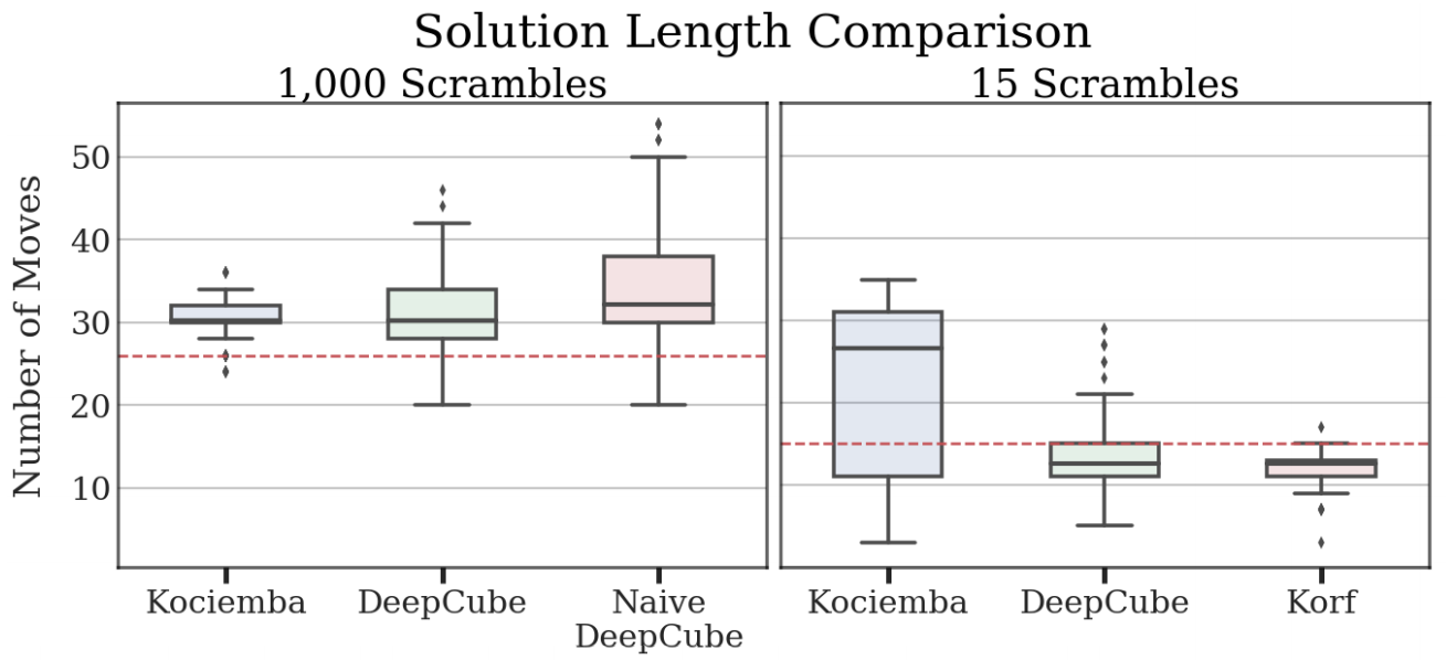
The final result published in the paper is quite impressive. After 44 hours of training on the machine with three GPUs, the network has learned how to solve cubes at the same level (and sometimes better) than human-crafted solvers. The final model has been compared against the two solvers described earlier: Kociemba two-staged solver and Korf IDA*. The method proposed in the paper is named DeepCube.

To compare the method efficiency, 640 randomly scrambled cubes are proposed to all methods. The depth of scramble was 1000 moves. The time limit for solution was 1 hour and both DeepCube and Kociemba solvers were able to solve all of the cubes within the limit. Kociemba solver is very fast, and its median solution time is just one second, but due to the manual rules, its solutions are not always the shortest ones. DeepCube method took much more time with median time is about 10 minutes, but was able to mach the length of Kociemba solutions or find better in 55% of cases. From my personal perspective, 55% is not enough to say that NNs are significantly better, but, at least it is not worse. On figure below, taken from the paper, the length
distributions for all solvers has been shown. As you can see, Korf solver wasn’t compared in 1000 scramble test cases, due to very long time to solve the cube. To compare performance of DeepCube against Korf solver, much easier, 15-steps scramble test set was created.

Implementation outline

Ok, now let’s switch to the code, which is available here. In this section I’m going to give a quick outline of my implementation and the key design decisions, but before that, I have to emphasize the important points about the code to set up the correct expectations.

• I’m not a researcher, so, the orginal goal of this code was just to reimplement the paper’s method. Unfortunately, the paper has very little details about the exact hyperparameters used, so, I was needed to guess and experiment a lot, and still, my results are very different from the published in the paper.
• At the same time, I’ve tried to implement everything in a general way to simplify further experiments. For example, the exact details about the cube state and transformations are abstracted away, which allows to implement more puzzles similar to 3x3 cube just by adding a new module. In my code, two cubes are implemented: 2x2 and 3x3, but any fully-observable environment with the fixed set of predictable actions is possible to implement and experiment with. Details are given in the next subsection.
• The code clarity and simplicity was put in front of performance. Of course, when it was possible to improve performance without introducing much overhead, I did so. For example, the training process was sped up by a factor of 5 by just splitting the generation of the scrambled cubes and forward network pass. But if performance required to refactor everything into multi-GPU and multi-threaded mode, I’d prefer to keep things simple. The very vivid example is MCTS process, which is normally implemented as a multi-threaded code, sharing the tree. It usually gets several times speed up, but requires tricky synchronization between processes. So, my version of MCTS is serial, with only trivial optimization of the batched search.

Overall, the code consists of the following parts:

1. Cube environment which defines observation space, possible actions and exact representation of the state to the network. This part is implemented in libcube/cubes module.
2. Neural Network part which describes the model we’ll train, generation of training samples and the training loop. It includes the training tool andlibcube/model.py module.
3. Solver of cubes, including the solver tool and libcube/mcts.py.
4. Various tools used to glue up other parts, like configuration files with hyperparameters and tools used to generate cube problemsets.

Cube environments

As we’ve already seen, combinatorial optimisation problems are quite large and diverse. Even the narrow area of cube-like puzzles include couple of dozens variations. The most popular ones are 2x2x2, 3x3x3, 4x4x4 Rubick’s cubes, Square-1, Pyraminx and tons of others. At the same time, the method presented in the paper is quite general and doesn’t depend on prior domain knowledge, amount of actions and state space size. The critical assumptions imposed on the problem include:

• States of the environment need to be fully observable and observations need to distinguish states from each other. That’s the case for the cube when we can see all the sides’ states, but doesn’t hold for most variants of a poker, for example, when we can’t see cards of our opponent.
• Amount of actions need to be discrete and finite. There are limited amount of actions we can do with the cube, but if our action space is “rotate the steering wheel on angle α ∈ [-120°…+120°]’’, we have different problem domain here.
• We need to have a reliable model of the environment, in other words, we have to be able to answer questions “what will be the result of applying action a to the state s?’’. Without this, both ADI and MCTS become non-applicable. This is a strong requirement and for most of the problems we don’t have such a model or its outputs are quite noisy. On the other hand, in games like chess or go we have such a model: rules of the game.
• In addition, our domain is deterministic, as the same action applied to the same state always ends up in the same final state. I have a feeling that methods should work even when we have stochastic actions, but I might be wrong.

To simplify application of the methods to domains different from 3x3 cube, all concrete environment details are moved in separate modules, communicating
with the rest of the code via abstract interface CubeEnv, which is available here. Every environment has a name, which should be specified to denote the concrete type of environment to be used. At the moment, two different environments are implemented: classical cube 3x3x3 with name cube3x3 and smaller one 2x2x2 with name cube2x2.

If you want to implement your own kind of cube or completely different environment all you need to do is to implement it following the interface and register it to make available for the rest of the code.

Training

Training process is implemented in tool train.py and module libcube/model.py. To simplify experimentation and make them reproducible, all the parameters of training are specified in a separate ini-file, which specifies the following options of training:

• Name of the environment to be used, currently cube2x2 and cube3x3 are available,
• Name of the run, which is used in TensorBoard names and directories to save models,
• What target value calculation method in ADI will be used. I’ve implemented two of them: one is described in the paper and my modification which, from my experiments, has more stable convergence,
• Training parameters: batch size, usage of CUDA, learning rate, LR decay and others.

You can find the examples of my experiments in the ini folder in repo.
During the training, TensorBoard metrics of the parameters are written in the runs folder. Models with the best loss value are being saved in the saves dir.

Search process

The result of the training is a model file with network’s weights. Those files could be used to solve cubes using MCTS, which is implemented in tool solver.py and module libcube/mcts.py.

Solver tool is quite flexible and could be used in various modes:

1. solve a single scrambled cube given as a comma-separated list of action indices, passed in -p option. For example -p 1,6,1 is a cube scrambled by applying the second action, then the seventh action and finally the second action again. The concrete meaning of actions is environment specific, which is passed with -e option. You can find actions with their indices in the cube environment module. For example, actions 1,6,1 for cube 2x2 mean L,R',L transformation.
2. read permutations from a text file (one cube per line) and solve them. File name is passed with -i option. There are several sample problems available in folder cubes_tests. You can generate your own problem sets using gen_cubes.py tool.
3. generate random scramble of the given depth and solve it
4. run series of tests with increasing complexity (scramble depth), solve them and write csv file with result. This mode is enabled by passing -o option and is very useful to evaluate the quality of the trained model. But it can take lots of time to complete. Optionally, plots with those test results are produced.

In all cases, you need to pass environment name with -e option and file with model’s weights (-m option). In addition, there are other parameters, allowing to tweak MCTS options and time or search step limits.

Experiment results

As I’ve already mentioned, I’m not a researcher, so, the original goal of this work was to reimplement the method from the paper and play with it. But, the paper provides no details about very important aspects of the method, like training hyperparameters, how deeply cubes were scrambled during the training, obtained convergence and lots of others. To get the details, I’ve sent an email to the paper authors, but never heard back from them.

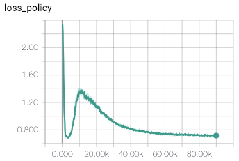
So, lots of experiments were required, and still my results are very different from the published in the paper. First of all, training convergence of the original method is very unstable. Even with small learning rate and large batch size, training eventually diverges, by having value loss component growing exponentially. Examples of this behaviour are shown on figure below.

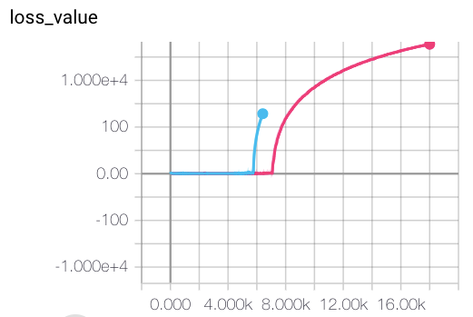
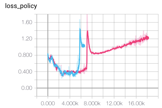
After several experiments with this, I’ve come to the conclusion, that this behaviour is a result of the wrong value objective, proposed in the method.
Indeed, in formula vᵢ = maxₐ(v(s, a) + R(A(s, a))), the value v(s, a) returned by the network is always added to the actual reward R(s), even for the goal state. With this, the actual values returned by the network could be anything: -100, 10⁶ or 3.1415. This is not a great situation for neural network training, especially with MSE value objective.

To check this, I modified the method of the target value calculation, by assigning zero target for the goal state:

This target could be enabled in ini file, by specifying param value_targets_method=zero_goal_value, instead of the default value_targets_method=paper.

With this simple modification, training process converged much quicker to stable values returned by value head of the network. The example of convergence is shown in figures below.

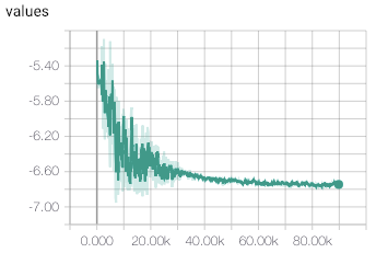
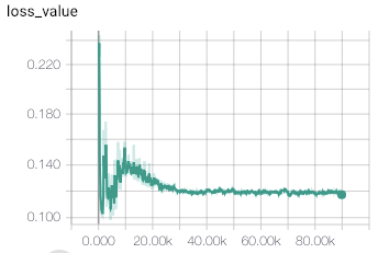
Cube 2x2

In the paper, authors reported training for 44 hours on a machine with three Titan XP GPUs. During the training, their model has seen 8 billions cube states. Those numbers correspond to training speed ≈50000 cubes/second. My implementation shows 15000 cubes/second on single GTX 1080Ti, which is comparable. So, to repeat the training process on a single GPU, we need to wait for almost 6 days, which is not very practical for experimentation and hyperparameter tuning.

To deal with this, I’ve implemented much simpler 2x2 cube environment, which takes just an hour to train. To reproduce my training, there are two ini files in the repo:

• cube2x2-paper-d200.iniuses value target method described in the paper,
• cube2x2-zero-goal-d200.inivalue target is set to zero for goal states.

Both configurations use batches of 10k states and scramble depth of 200. Training params are the same.

After the training, using both configuration, two models were produced
(both are stored in the repo):

• paper method: loss 0.18184,
• zero goal method: loss 0.014547.

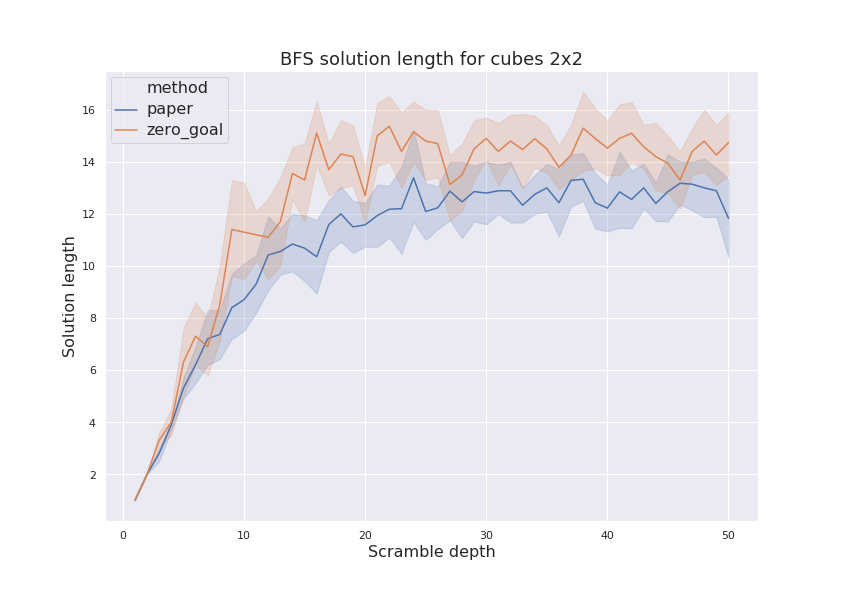
My experiments (using solver.py utility) has shown that model with lower loss has much higer success ratio of solving randomly-scrambled cubes of increasing depth. Results for both models are shown on figure.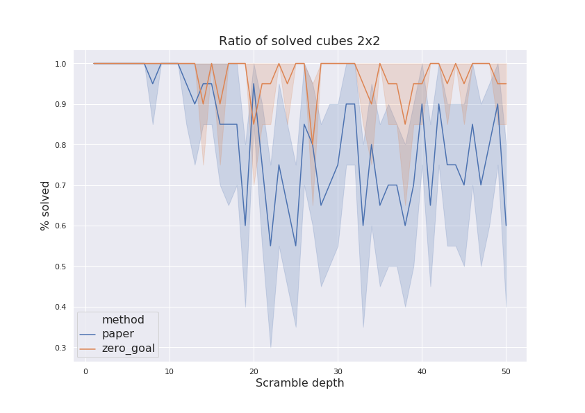

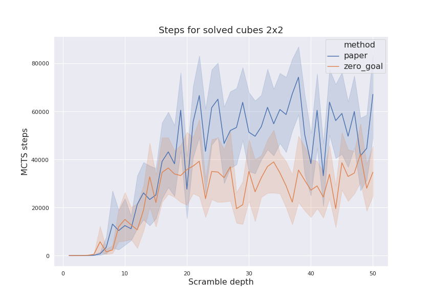
Next parameter to compare is amount of MCTS steps done during the solution. It has shown on figure below and zero goal model normally finds solution in less amount of steps. In other words, the policy it has learned is better.

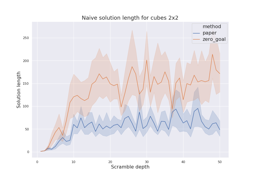
And, finally, let’s check the length of found solutions. On figure below, both naïve and BFS solution lengths are plotted. From those plots it could be seen that naïve solutions length are much longer (by a factor of 10) than solutions found by BFS. Such a difference might be an indication of untuned MCTS parameters which could be improved. “Zero goal’’ model shows longer solutions than “paper’’ model, as the former fails to find longer solutions at all.

Cube 3x3

Training of 3x3 cube model is much more heavy, so, probably I’ve just scratched the surface here. But even my limited experiments shows that
zero-goal modifications to the training method greatly improves training stability and resulting model quality. But training requires now about 20 hours, so, running lots of experiments require time and patience.

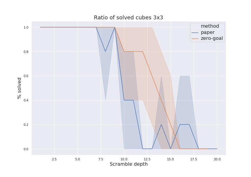
My results are not that shiny as reported in the paper: the best model I was able to obtain can solve cubes up to scrambling depth of 12…15, but consistently fails for more complicated problems. Probably, those numbers could be improved with more CPU cores + parallel MCTS. To get the data, search process was limited in 10 minutes and for every scramble depth, five random scrambles were generated.

Figure below shows comparison of solution rates for method presented in the paper and modified version with zero value target.

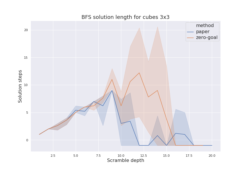
The final figure shows length of optimal solution found. There are two interesting issues could be noted there. First of all, length of solutions found by “zero target’’ method in 10…15 scramble depth range is larger than scramble depth. This means that model failed to find scramble sequence used to generate test problem, but still discovered some longer way. Another thing is that for depth range 12…18, “paper’’ method found solutions which where shorter than scramble sequence. This could happen due to degenerate test sequence was generated.

Further improvements and experiments

There are lots of directions and things could be tried to make the results better. Something from the top of my head:

• More input and network engineering. Cube is a complicated thing, so, simple feed-forward NNs could be not the best model. Probably network could greatly benefit from convolutions.
• Oscillations and instability during the training might be the signal of common RL issue with inter-step correlations. The usual approach is target network, when we’re using old version of network to get bootstrapped values.
• Priority replay buffer might help for training speed.
• My experiments shows that samples weighting (inverse proportional to scramble depth) helps to get better policy which knows how to solve
   slightly scrambled cubes, but might slow down the learning of more deep states. Probably, this weighting could be made adaptive to make it less aggressive in later training stages.
• Entropy loss could be added to training to regularize our policy.
• Cube 2x2 model doesn’t take into account that cube doesn’t have central cubelets, so, the whole cube could be rotated. This might be not very important for 2x2, as states space is small, but the same observation will be critical for 4x4 cubes.
• Definitely, more params tuning are needed to get better training and MCTS params.