Up and running with PyTorch — minibatching, dataloading and model building

Published by: Conor McDonald

I have now experimented with several deep learning frameworks — TensorFlow, Keras, MxNet — but, PyTorch has recently become my tool of choice. This isn’t because I think it is objectively better than other frameworks, but more that it feels pythonic, intuitive, and better suited to my style of learning and experimenting.

This post provides a tour around PyTorch with a specific focus on building a simple neural network (feed forward network) to separate (i.e. classify) two classes in some toy data. My goal is to introduce some of PyTorch’s basic building blocks, whilst also highlighting how deep learning can be used to learn non-linear functions. All of the code for this post is this github repo. This is more of a practical post, if you are looking for a tour of the inner workings of PyTorch I strongly recommend this post.

To follow along make sure you have PyTorch installed on your machine. Note that I am using version 0.3.1.post2 The next version of pytorch (0.4) will introduce some breaking changes (read about them here). Also worth keeping an eye out for the release of PyTorch 1.0, which aims to be “production ready” — I’m very excited for this!.

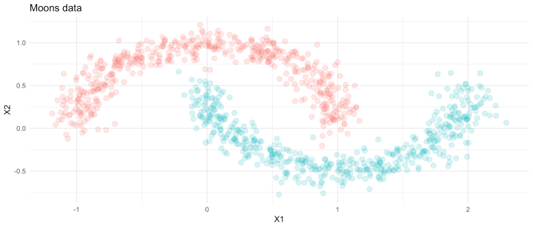
The learning task for this post will be a binary classification problem — classifying points in half moon shapes. This is a simple task for a deep learning model, but it serves to highlight their ability to learn complex, non-linear functions.

For example, if we use a logistic regression to classify this data look what happens:

from sklearn.datasets import make_moons
	import pandas as pd
	import numpy as np
	import torch
	from torch.autograd import Variable
	import torch.nn as nn
	from torch.utils.data import Dataset, DataLoader
	import torch.nn.functional as F
	def to_categorical(y, num_classes):
	"""1-hot encodes a tensor"""
	return np.eye(num_classes, dtype='uint8')[y]
	X, y = make_moons(n_samples=1000, noise=.1)
	y = to_categorical(y_, 2)

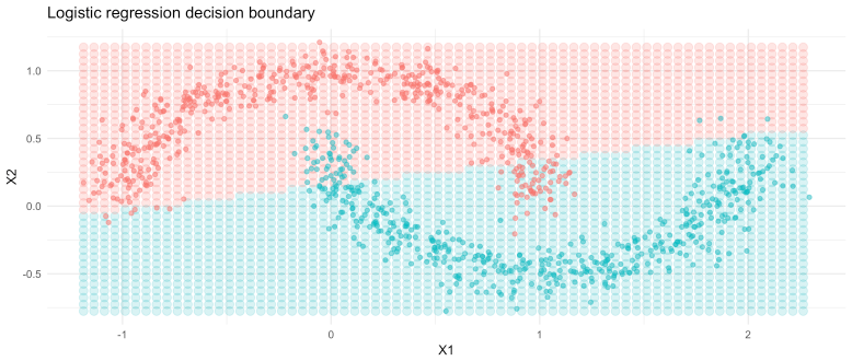
Despite applying a softmax transformation to the predicted outputs (squeezing predicted output logits to sum to 1), the logistic regression is linear in its parameters and, therefore, struggles to learn non-linear relationships. We could use a more advanced ML model for this task, such as a random forest, but then we wouldn’t have an excuse to play around with a neural network!

Before building the model, we will first create a custom data pre-processor and loader. In this example, the transformer will simply transform X and y from numpy arrays to torch tensors. We will then use the dataloader class to handle how data is passed through the model. Note that we have to define __len__ and __getitem__ methods for this class.

class PrepareData(Dataset):
	def __init__(self, X, y):
	if not torch.is_tensor(X):
	self.X = torch.from_numpy(X)
	if not torch.is_tensor(y):
	self.y = torch.from_numpy(y)
	def __len__(self):
	return len(self.X)
	def __getitem__(self, idx):
	return self.X[idx], self.y[idx]
	ds = PrepareData(X=X, y=y)
	ds = DataLoader(ds, batch_size=50, shuffle=True)

In this instance we will set-up a mini-batch routine. This means that during each epoch the model will train on small subsets (batches) of the data — that is, it will update its weights with respect to the loss associated with each mini-batch. This is generally a better approach than training on the full dataset each epoch. It is also advisable to use smaller batches — though this is a hyper parameter so do experiment!

Defining a model

The standard approach to defining a deep learning model with PyTorch is to encapsulate the network in a class. I quite like this approach because it ensures that all layers, data, and methods are accessible from a single object. The purpose of the class is to define the architecture of the network and to manage the forward pass of the data through it. To define the model we need to inherit the nn.Module.

The typical approach is to define layers as variables. In this case we define a single layer network. The nn.Linear function requires input and output size. In the first layer input size is the number the features in the input data which in our contrived example is two, out features is the number of neurons the hidden layer.

class MoonsModel(nn.Module):
	def __init__(self, n_features, n_neurons):
	super(MoonsModel, self).__init__()
	self.hidden = nn.Linear(in_features=n_features, out_features=n_neurons)
	self.out_layer = nn.Linear(in_features=n_neurons, out_features=2)
	def forward(self, X):
	out = F.relu(self.hidden(X))
	out = F.sigmoid(self.out_layer(out))
	return out

The input to the output layer is the number of neurons in the previous layer and the output is the number of targets in the data — in this case two.

We then define a class method forward to manage the flow of data through the network. Here we call the layers on the data and also use apply the reluactivation (from torch.nn.functional) on the hidden layer. Finally, we apply a sigmoid transformation on the output to squeeze the predicted values to sum to one.

Running the model

Next we need to define how the model learns. First we instantiate a model object from the class, we’ll call this model. Next we define the cost function – in this case binary cross entropy – see my previous post on log loss for more information. Finally we define our optimiser, Adam. The optimiser will be optimising parameters of our model, therefore, the params argument is simply the model parameters.

Now we are ready to train the model. We will do this for 50 epochs. I have commented the code block to make it clear what is happening at each stage. We set up a for loop to iterate over the data (epochs) and with each epoch we loop over the mini batches of X and y stored in ds, which we defined previously. During each of these loops we make the input and target torch Variables (note this step will not be necessary in the next release of pytorch because torch.tensors and Variables​ will be merged) and then specify the forward and backward pass.

The forward pass uses the model parameters to predict the outputs. In this first pass the prediction will be close to random because the parameters are initialized with random numbers. In this pass we calculate loss associated with the model using the cost function we instantiated.

model = MoonsModel(n_features=2, n_neurons=50)
	cost_func = nn.BCELoss()
	optimizer = tr.optim.Adam(params=model.parameters(), lr=0.01)
	num_epochs = 20
	losses = []
	accs = []
	for e in range(num_epochs):
	for ix, (_x, _y) in enumerate(ds):
	#=========make inpur differentiable=======================
	_x = Variable(_x).float()
	_y = Variable(_y).float()
	#========forward pass=====================================
	yhat = model(_x).float()
	loss = cost_func(yhat, _y)
	acc = tr.eq(yhat.round(), _y).float().mean() # accuracy
	#=======backward pass=====================================
	optimizer.zero_grad() # zero the gradients on each pass before the update
	loss.backward() # backpropagate the loss through the model
	optimizer.step() # update the gradients w.r.t the loss
	losses.append(loss.data[0])
	accs.append(acc.data[0])
	if e % 1 == 0:
	print("[{}/{}], loss: {} acc: {}".format(e,
	num_epochs, np.round(loss.data[0], 3), np.round(acc.data[0], 3)))

In the forward pass we use to model to predict y given X, calculate the loss (and accuracy). To so so we just pass the data through the model. In the backward pass we backproprogate the loss through the model and optimiser.step updates the weights according to the learning rate.

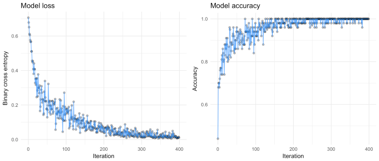
We can see that the loss decreases rapidly (the volatility can be explained by the mini-batches), which means our model is working — awesome! You can also see the non-linear decision regions learned by the model.

Also, check out the decision regions learned by the model:

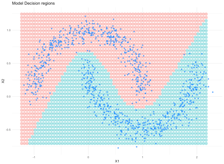
It is pretty clear that the neural network can learn the non-linear nature of the data!

Explanation on Neural Arithemetic Logical Units

Neural Arithmetic Logic Units (NALU): Explanation, Intuition and Code

Published By: Faizan Patel

The research engineers at DeepMind including well known AI researcher and author of the book Grokking Deep Learning, Andrew Trask have published an impressive paper on a neural network model that can learn simple to complex numerical functions with great extrapolation (generalisation) ability.

In this post I will explain NALU, its architecture, its components and significance over traditional neural networks. The primary intention behind this post is to provide simple and intuitive explanation of NALU (both with concepts and code) which can be comprehended by researchers, engineers and students who have a limited knowledge of neural networks and deep learning.

---

Where do Neural Networks fail?

This image is taken from this medium post

Neural networks, in theory, are very good function approximators. They can almost always learn any meaningful relationship between inputs (data or features) and outputs (labels or targets). Hence, they are being used in a wide variety of applications from object detection and classification to speech to text conversion to intelligent game-playing agents that can beat human world champion players. There are many effective neural network models which satisfied various need of such applications such as Convolutional Neural Networks (CNNs), Recurrent Neural Networks (RNNs), Autoencoders etc. Advances in deep learning and neural network models is another topic in itself.

However, according to the authors of the paper, they lack very basic ability which seems trivial for a human or for even bees! That is the ability to count/manipulate numbers and also, to extrapolate the numerical relationship from an observable numeric pattern. In the paper, it is shown that the standard neural networks even struggles to learn even an identity function ( a function whose input and output is identical; f(x) = x) which is the most straightforward numeric relationship. Below image shows the mean square error (MSE) of various NNs trained to learn such an identity function.

The Image shows the MSE for a standard Neural Network having exact same architecture trained using different activation functions (non-linearaity) in the hidden layers

Why they fail?

The primary reason for NNs to fail to learn such numerical representation is the use of non linear activation functions in hidden layers of the network. Such activation functions are crucial to learn the abstract non linear relationship between inputs and labels but they fail miserably when it comes to learn the numerical representation outside the range of the numbers seen in the training data. Hence, such networks are very good to memorize the numerical pattern seen in the training set but fail to extrapolate this representation well.

It is like memorizing an answer or a topic without understanding the underlying concept for the exam. Doing so, one can perform very well if the similar questions are asked in the exam, however, would fail in the case of twisted questions are asked designed to test the knowledge and not the memorization ability of a candidate.

The severity of this failure directly corresponds to the degree of non-linearity within the chosen activation function. From the above image, it can be clearly seen that the hard-constrained non-linear functions such as Tanh and Sigmoid have very less ability to generalize well than the soft-constrained non-linear function such as PReLU and ELU.

Solution: Neural Accumulator (NAC)

The neural accumulator (NAC) forms the base to the NALU model. NAC is a simple but effective neural network model (unit) which supports the ability to learn addition and subtraction — which is a desirable property to learn linear functions effectively.

NAC is a special layer of linearity whose weight parameters have the restrictions of having the only values 1, 0 or -1. By constraining the weight values in such a manner prevents the layer from changing the scale of the input data and they remain consistent throughout the network no matter how many layers are stacked together. Hence, the output will be the linear combination of input vector which can easily represent addition and subtraction operations.

Intuition: To understand this fact, let us consider the following examples of NN layers which performs the linear arithmetic operation on inputs.

Illustration to explain that the Neural network layers with no bias and having weights value -1, 0 or 1 can learn linear extrapolation.

As shown in above NN layers, network can learn to extrapolate simple arithmetic functions like addition and subtraction ( y= x1 + x2 and y = x1—x2) by restricting the weight parameters to -1, 0 and 1.

Note: As shown in the network diagrams above, NAC contains no bias parameter (b) and no non-linearity applied to the output of hidden layer units.

Since the constraint on the weight parameters in NAC is hard to learn by standard neural network, authors have described very useful formula to learn such restricted parameter values using standard (unconstrained) parameters W_hat and M_hat. These parameters are like any standard NN weight parameters which can be initialized randomly and can be learnt over the course of training process. The formula to obtain W in terms of W_hat and M_hat is given below:

Formula denotes the element-wise product between two matrices

Using above equation to calculate the weight parameters in the network, guarantees that the value of such parameters will be in the range of [-1,1] with more inclined towards -1, 0 and 1. Also, this equation is a differentiableequation (whose derivatives can be computed with respect to weight parameters). Hence, it will be easier for NAC to learn W using gradient descent and back propagation. Below is the architectural diagram of a NAC unit.

NAC architecture to learn simple (linear) numeric functions

NAC implementation in python using Tensorflow

As one can imagine, NAC is a simple NN model with few little tweaks. Below I have shown the simple implementation of a single NAC layer in python using Tensorflow and Numpy library.

import numpy as np
import tensorflow as tf

# Define a Neural Accumulator (NAC) for addition/subtraction -> Useful to learn the addition/subtraction operation
def nac_simple_single_layer(x_in, out_units):

    '''
    Attributes:
        x_in -> Input tensor
        out_units -> number of output units

    Return:
       y_out -> Output tensor of mentioned shape
       W -> Weight matrix of the layer

    '''

# Get the number of input features (numbers)
    in_features = x_in.shape[1]

    # define W_hat and M_hat

    W_hat = tf.get_variable(shape=[in_features, out_units],
    initializer= tf.initializers.random_uniform(minval=-2,maxval=2),
    trainable=True, name="W_hat")

    M_hat = tf.get_variable(shape=[in_shape, out_units],
    initializer= tf.initializers.random_uniform(minval=-2,maxval=2),
    trainable=True, name="M_hat")

    # Get W using the formula
    W = tf.nn.tanh(W_hat) * tf.nn.sigmoid(M_hat) 

    y_out = tf.matmul(x_in, W)

    return y_out,W

In the above code, I used random uniform initialization for trainable parameters W_hat and M_hat but one can use any recommended weight initialization technique for these parameters. For full working code kindly checkout my GitHub repo mentioned at the end of this post.

Moving beyond addition and subtraction: NAC for complex numeric functions

Though the above mentioned simple neural network model is able to learn basic arithmetic functions like the addition and subtraction, it is desirable to have the ability to learn more complex arithmetic operations such as multiplication, division and power functions.

Below is the modified architecture of NAC that is able to learn more complex numeric functions using the log space (logarithmic values and exponents)for its weight parameters. Observe that how this NAC is different than the one mentioned first in the post.

NAC architecture to learn more complex numeric function

As shown in the diagram above, this cell applies the log function to the input data before matrix multiplication with weight matrix W and then it applies an exponential function on the resultant matrix. The formula to obtain output is given in the below equation.

Output equation of the complex NAC shown above. Epsilon here is a very small value to avoid log (0) situation during training

Hence, everything is same in terms of the underlying mechanism of simple NAC and complex NAC including the formula for restricted weights W in terms of W_hat and M_hat. The only difference is that complex NAC applies log space on input and output of the layer.

Python implementation of complex NAC:

As with the architectures of both NACs, the python implementation of complex NAC is almost same except mentioned change in the output tensor formula. Below is the code for such NAC.

# define a complex NAC in log space -> for more complex arithmetic functions such as multiplication, division and power
def nac_complex_single_layer(x_in, out_units, epsilon = 0.000001):

    '''
    :param x_in: input feature vector
    :param out_units: number of output units of the cell
    :param epsilon: small value to avoid log(0) in the output result
    :return m: output tensor
    :return W: associated weight matrix
    
    '''

    in_features = x_in.shape[1]

    W_hat = tf.get_variable(shape=[in_shape, out_units],
    initializer= tf.initializers.random_uniform(minval=-2,maxval=2),
    trainable=True, name="W_hat")

    M_hat = tf.get_variable(shape=[in_features, out_units],
    initializer= tf.initializers.random_uniform(minval=-2,maxval=2),
    trainable=True, name="M_hat")

    #Get Unrestricted parameter matrix W
    W = tf.nn.tanh(W_hat) * tf.nn.sigmoid(M_hat)

    # Express Input feature in log space to learn complex functions
    x_modified = tf.log(tf.abs(x_in) + epsilon)

    m = tf.exp( tf.matmul(x_modified, W) )

    return m, W

Once again, for full working code please checkout my GitHub repo mentioned at the end of this post.

Putting it all together: Neural Arithmetic Logic Units (NALU)

By now one can imagine that above two NAC models combined together can learn almost all arithmetic operations. That is the key idea behind NALU which comprises the weighted combination of a simple NAC and a complex NAC mentioned above, controlled by a learned gate signal. Thus, NAC forms the basic building block of NALUs. So, if you have understood the NAC properly, NALU is very easy to grasp. If you haven’t, please take your time and go through the both NAC explanations once again. Below image describes the architecture of NALU.

Annotated diagram of NALU

As shown in the above image, in NALU both NACs (purple cells) are interpolated (combined) by a learned sigmoid gate control (orange cell) such that the output of either NAC can be activated or deactivated by gate based on the numeric function we are trying to train the network for.

As mentioned above, the simple NAC computes the accumulation function so it is responsible to store NALU’s linear (addition and subtraction) operations. While the complex NAC is responsible to carry out its more complex numeric functions such as multiplication, division and power functions. The output of the underlying cells in an NALU can be represented mathematically as follows:

Simple NAC : a = W X

Complex NAC: m = exp ( W log (|X| + e) )

Where, W = tanh(W_hat) * sigmoid(M_hat)

Gate cell: g = sigmoid(GX) # Where G is standard trainable parameter matrix

# And finally the output of the NALU
NALU: y = g * a + (1-g) * m   # Where * is the element wise product

In the above formula of NALU, we can say that if gate output g=0 then the network will learn only complex functions but not the simple ones. In contrast, if g=1 then the network will learn only additive functions and not the complex ones. Hence, altogether NALU can learn any numeric functions consisting of multiplication, addition, subtraction, division, and power functions in such a way that extrapolates well to the numbers outside of the range of numbers that have been seen during training.

Python implementation of NALU:

In the implementation of NALU, we will use both simple and complex NAC defined in the previous code snippets.

def nalu(x_in, out_units, epsilon=0.000001, get_weights=False):
    '''
    :param x_in: input feature vector
    :param out_units: number of output units of the cell
    :param epsilon: small value to avoid log(0) in the output result
    :param get_weights: True if want to get the weights of the model 
                        in return
    :return: output tensor
    :return: Gate weight matrix
    :return: NAC1 (simple NAC) weight matrix
    :return: NAC2 (complex NAC) weight matrix
    '''

    in_features = x_in.shape[1]

    # Get the output tensor from simple NAC
    a, W_simple = nac_simple_single_layer(x_in, out_units)

    # Get the output tensor from complex NAC
    m, W_complex = nac_complex_single_layer(x_in, out_units,     epsilon= epsilon)

    # Gate signal layer
    G = tf.get_variable(shape=[in_features, out_units],
    initializer= tf.random_normal_initializer(stddev=1.0),
    trainable=True, name="Gate_weights")

    g = tf.nn.sigmoid( tf.matmul(x_in, G) )

    y_out = g * a + (1 - g) * m

    if(get_weights):
        return y_out, G, W_simple, W_complex
    else:
        return y_out

Again, in the above code, I used random normal initialization for gate parameters G but one can use any recommended weight initialization technique.

---

Ibelieve NALU is a modern breakthrough in AI and specifically in neural networks that seems very promising. They can open doors to many applications which seem to be difficult for standard NNs to deal with.

Authors have shown various experiments and results implementing NALU in different area of neural network applications in the paper from simple arithmetic function learning tasks to counting the number of handwritten digits in provided series of MNIST images to make the network learning to evaluate computer programs!

The results are amazing and prove that the NALU excel to generalize well in almost all tasks involving numerical representation than the standard NN models. I recommend readers to have a look at these experiments and its results to gain the deeper understanding of how NALU can be useful in some interesting numerical tasks.

However, it is unlikely that NAC or NALU will be the perfect solution for every task. Rather, they demonstrate a general design strategy for creating models that are intended for a target class of numerical functions.

---