Building your First Neural Network on a Structured Dataset (using Keras)

Published By:Sunil Ray

Introduction

Have you ever applied a neural network model on a structured dataset? If the answer is no, which of the following reasons are applicable for you?

1. It is very complex to apply
2. Neural Network is good for unstructured datasets like image, audio, and text and it does not perform well on structured datasets
3. It is not as easy as building a model using scikit-learn/caret
4. Training time is too high
5. Requires high computational power

In this article, I will focus on the first three reasons and showcase how easily you can apply a neural network model on a structured dataset using a popular high-level library - “keras”.

Understand the problem statement

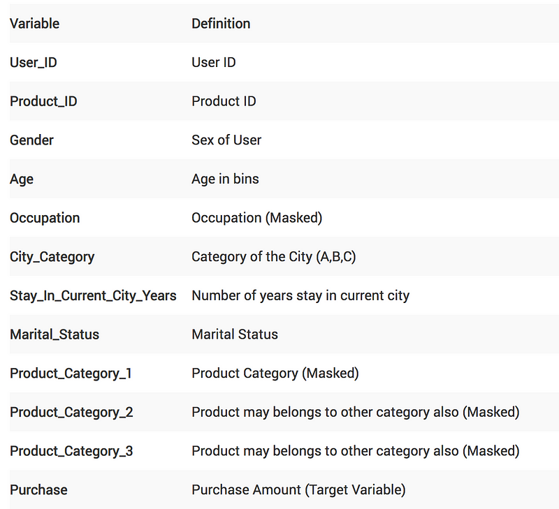
We will work on the Black Friday dataset in this article. It is a regression challenge where we need to predict the purchase amount of a customer against various products. We have been provided with various information about customer demographics (age, gender, marital status, city_type, stay_in_current_city) and product details (product_id and product category). Below is the data dictionary:

The evaluation metric for this challenge is theRoot Mean Squared Error (RMSE).

Pre-requisite

In this article, I will solve this Black-Friday challenge using a Random Forest (RF) model using scikit-learn and a basic Neural Network (NN) model using keras. The idea of this article is to show how easily we can build an NN model on a structured dataset (it is similar to building a RF model using the scikit-learn library). This article assumes that you have a fair background of building a Machine Learning model, scikit-learn, and the basics of Neural Network. If you are not comfortable with these concepts, I would recommend going through the below articles first:

1. Introduction-deep-learning-fundamentals-neural-networks
2. Understanding-and-coding-neural-networks-from-scratch-in-python
3. Common Machine Learning Algorithms

Approach to solve the problem using Machine (Deep) learning

I’m going to separate my approach broadly into four sub-sections:

1. Data Preparation
2. Model Building (Random Forest and Neural Network)
3. Evaluation
4. Prediction

Data Preparation

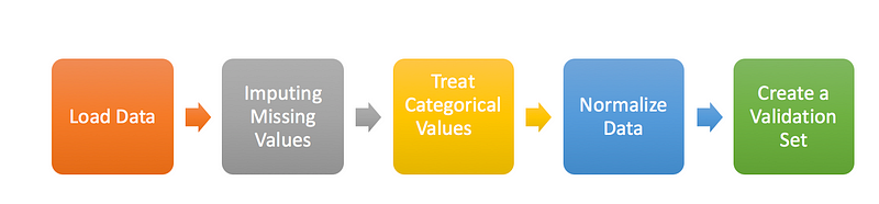
In this section, I will focus on basic data preparation steps like loading the dataset, imputing missing values, treating categorical variables, normalizing data and creating a validation set. I will follow the same steps for both the Random Forest and our NN model.

• Load Data: Here, I’ll import the necessary libraries to load the dataset, combine train and test to perform preprocessing together, and also create a flag for the same.

#Importing Libraries for data preparation
import pandas as pd
import numpy as np

#Read Necessary files
train = pd.read_csv("train_black_friday.csv")
test = pd.read_csv("test_black_friday.csv")

#Combined both Train and Test Data set to do preprocessing together # and set flag for both as well
train['Type'] = 'Train' 
test['Type'] = 'Test'
fullData = pd.concat([train,test],axis=0)

• Impute Missing Values: Methods to treat missing values for categorical and continuous variables will be different.
  So, our first step would be identifying the ID column, target variable, categorical and continuous independent variables.
  Post this, we will create dummy flags for missing value(s). Why do this? Because sometimes missing values themselves can carry a good amount of information. Finally, we will impute the missing values of continuous variables with the mean of that columns, and for the categorical variable, we will create a new level.

#Identifying ID, Categorical
ID_col = ['User_ID','Product_ID']
flag_col= ['Type']
target_col = ["Purchase"]
cat_cols= ['Gender','Age','City_Category','Stay_In_Current_City_Years']
num_cols= list(set(list(fullData.columns))-set(cat_cols)-set(ID_col)-set(target_col)-set(flag_col))

# Combined numerical and Categorical variables
num_cat_cols = num_cols+cat_cols

#Create a new variable for each variable having missing value with VariableName_NA 
# and flag missing value with 1 and other with 0

for var in num_cat_cols:
    if fullData[var].isnull().any()==True:
        fullData[var+'_NA']=fullData[var].isnull()*1

#Impute numerical missing values with mean
fullData[num_cols] = fullData[num_cols].fillna(fullData[num_cols].mean())

#Impute categorical missing values with -9999
fullData[cat_cols] = fullData[cat_cols].fillna(value = -9999)

• Treat Categorical Values: We will create a label encoder for categorical variables.

#create label encoders for categorical features
from sklearn.preprocessing import LabelEncoder

for var in cat_cols:
    number = LabelEncoder()
    fullData[var] = number.fit_transform(fullData[var].astype('str'))

• Normalize Data: Scale (normalize) the independent variables between 0 and 1. It will help us to converge comparatively faster.

features = list(set(list(fullData.columns))-set(ID_col)-set(target_col))
fullData[features] = fullData[features]/fullData[features].max()

• Create a validation Set: Here, we will segregate the train-test from the full dataset and remove the train-test flag from features list. While building our model, we have target values for the train dataset only, so we will create a validation set out of this train dataset for evaluating the model’s performance. Here, I’m using train_test_split to divide the train dataset in training and validation in a 70:30 ratio.

#Creata a validation set
from sklearn.model_selection import train_test_split

train=fullData[fullData['Type']==1]
test=fullData[fullData['Type']==0]
features=list(set(list(fullData.columns))-set(ID_col)-set(target_col)-set(flag_col))

X = train[features].values
y = train[target_col].values

X_train, X_valid, y_train, y_valid = train_test_split(X, y, test_size=0.30, random_state=42)

Model Building using Random Forest

This part is fairly straightforward and I have written about this multiple times before. If you still want to review the random forest algorithm and its parameters, I would recommend going through this article: Tutorial on Tree Based Algorithms.

#import necessary libraries to build model

import random
from sklearn.ensemble import RandomForestRegressor

random.seed(42)
rf = RandomForestRegressor(n_estimators=10)
rf.fit(X_train, y_train)

Model Building using Deep Learning Model (Keras)

Here, I will focus on the steps to build a basic deep learning model. This will help beginners in creating their own models in the future. The steps to do this are:

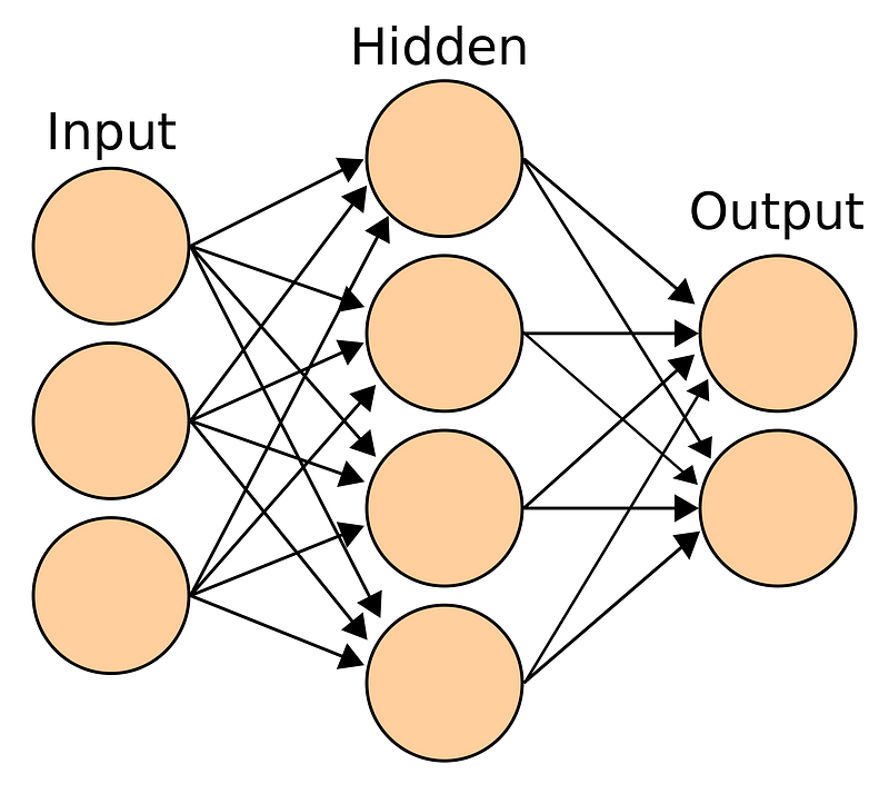
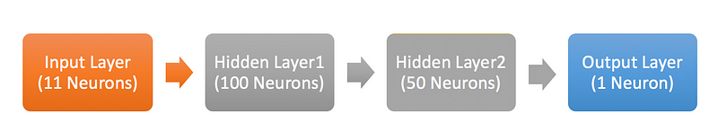
• Define Model: For building a deep learning model, we need to define the layers (Input, Hidden, and Output). Here, we will go ahead with a sequential model, which means that we will define layers sequentially. Also, we will be going ahead with a fully connected network.
  1. First, we will focus on defining the input layer. This can be specified while creating the first layer with the input dim argument and setting it to 11 for the 11 independent variables.
  2. Next, define the number of hidden layer(s) along with the number of neurons and activation functions. The right number can be achieved by going through multiple iterations. Higher the number, more complex is your model. To start with, I’m simply using two hidden layers. One has 100 neurons and the other has 50 with the same activation function - “relu”.
  3. Finally, we need to define the output layer with 1 neuron to predict the purchase amount. The problem in hand is a regression challenge so we can go ahead with a linear transformation at the output layer. Therefore, there is no need to mention any activation function (it is linear by default).

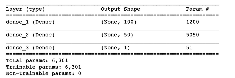
# Define model
model = Sequential()
model.add(Dense(100, input_dim=11, activation= "relu"))
model.add(Dense(50, activation= "relu"))
model.add(Dense(1))
model.summary() #Print model Summary

• Compile Model: At this stage, we will configure the model for training. We will set the optimizer to change the weights and biases, and the loss function and metric to evaluate the model’s performance. Here, we will use “adam” as the optimizer, “mean squared error” as the loss metric. Depending on the type of problem we are solving, we can change our loss and metrics. For binary classification, we use “binary-crossentropy” as a loss function.

# Compile model
model.compile(loss= "mean_squared_error" , optimizer="adam", metrics=["mean_squared_error"])

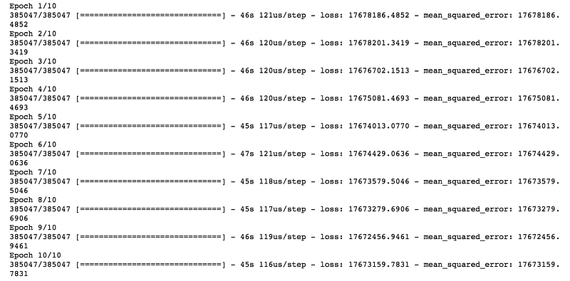
• Fit Model: Now, the final step of model building is fitting the model on the training dataset (which is actually 70% of the full dataset). We need to provide both independent and dependent variables along with the number of training iterations, i.e. epochs. Here, we have taken 10 epochs.

# Fit Model
model.fit(X_train, y_train, epochs=10)

Evaluation

Now that we have built the model using Random Forest and Neural Network techniques, the next step is to evaluate the performance on the validation dataset for both the models.

• Evaluation for Random Forest Model: We will get the predictions on the validation dataset and do the evaluation with actual target values (y_valid). We get the root mean squared error as ~3106.

from sklearn.metrics import mean_squared_error
pred=rf.predict(X_valid)
score = np.sqrt(mean_squared_error(y_valid,pred))
print (score)
3106.5008973291074

# Evaluation while fitting the model
model.fit(X_train, y_train, epochs=10, validation_data=(X_valid, y_valid))

• Evaluation for Neural Network Model: Similarly, we will get the predictions on the validation dataset using the neural network model and calculate the root mean squared error. RMSE with a basic NN model comes out to be ~4214. This is a fairly basic model, you can go ahead and tune the hyper-parameters to build a more complex network. You can pass validation data as an argument while fitting the NN model as well to look at the validation score after each epoch.

pred= model.predict(X_valid)
score = np.sqrt(mean_squared_error(y_valid,pred))
print (score)
4213.954523194906

Prediction

After evaluating the model and finalizing the model parameters, we can go ahead with the prediction on the test data. Below is the code to do this using both random forest and NN models.

#Select the independent variables for test dataset
X_test = test[features].values

#Prediction using Random Forest 
y_test_rf = rf.predict(X_test)

#Prediction using Neural Network
y_test_nn = model.predict(X_test)

What’s Next

The idea of this article was to show how easily we can build an NN model on a structured dataset so we have not focused on other aspects of improving the model’s predictions. Below is my list of ideas which you can apply to build on the neural network:

• Impute missing values after looking at the variable to variable relationships
• Feature Engineering (Product Ids may have some information about the purchase amount)
• Select right hyper-parameters
• Build a more complex network by adding more hidden layers
• Use regularization
• Train for more number of epochs
• Take Ensemble of both RF with NN model

Summary

In this article, we have discussed the different stages of model building like data preparation, model building, evaluation and finally prediction. We also looked at how we can apply a neural network model on a structured dataset using keras.

PinSage: A New Graph Convolutional Neural Network for Web-Scale Recommender Systems

Ruining He | Pinterest engineer, Pinterest Labs

Deep learning methods have achieved unprecedented performance on a broad range of machine learning and artificial intelligence tasks like visual recognition, speech recognition and machine translation. However, despite amazing progress, deep learning research has mainly focused on data defined on Euclidean domains, such as grids (e.g., images) and sequences (e.g., speech, text). Nonetheless, most interesting data, and challenges, are defined on non-Euclidean domains such as graphs, manifolds and recommender systems. The main question is, how to define basic deep learning operations for such complex data types. With a growing and global service, we don’t have the option of a system that won’t scale for everyday use. Our answer came in the form of PinSage, a random-walk Graph Convolutional Network capable of learning embeddings for nodes in web-scale graphs containing billions of objects.

Here we’ll show how we can create high-quality embeddings (i.e. dense vector representations) of nodes (e.g., Pins/images) connected into a large graph. The benefit of our approach is that by borrowing information from nearby nodes/Pins the resulting embedding of a node becomes more accurate and more robust. For example, a bed rail Pin might look like a garden fence, but gates and beds are rarely adjacent in the graph. Our model relies on this graph information to provide the context and allows us to disambiguate Pins that are (visually) similar, but semantically different.

To our knowledge, this is the largest application of deep graph embeddings to date and paves the way for a new generation of web-scale recommender systems based on graph convolutional architectures.

Background

One of Pinterest’s greatest values is our ability to make visual recommendations based on taste by taking into account the context added by hundreds of millions of users, and then to help people discover ideas and products that match their interests. As the number of people using Pinterest grows beyond 200M+ MAU, and the number of objects saved has crossed 100B, we must continuously build technology to not only keep up, but make recommendations smarter.

As a content discovery application, people use Pinterest to save and organize Pins, which are visual bookmarks to online content (recipes, clothes, products, etc.) onto boards. We model the Pinterest environment as a bipartite graph consisting of nodes in two disjoint sets, Pins and boards. Each Pin is associated with certain information like an image and a set of textual annotations (title, description). Here we aim to generate high-quality embeddings of Pins from our bipartite graph with visual and annotation embeddings as input features.

Pin embeddings are essential to various tasks like recommendation of Pins — including dynamic Pins like those for ads, and shopping — classification, clustering, and even reranking. Such tasks are fundamental to our key services like Related Pins, Search, Shopping, Ads. To achieve our goal of generating high-quality embeddings, we developed a highly-scalable, generic deep learning model called PinSage to extract embeddings of nodes from web-scale graphs. We have successfully applied PinSage on Pinterest data with billions of nodes and tens of billions of edges.

Challenges

In recent years, Graph Convolutional Networks (GCNs) have been proposed to model graphs and seen success on various recommender systems benchmarks. However, these gains on benchmark tasks have yet to be translated to gains in real-world production environments. The main challenge is to scale both the training as well as inference of GCN-based node embeddings to graphs with billions of nodes and tens of billions of edges. Scaling up GCNs is difficult because many of the core assumptions underlying their design are violated when working in a big data environment. For example, all existing GCN-based recommender systems require operating on the full graph Laplacian during training — an assumption that is infeasible when the underlying graph has billions of nodes and whose structure is constantly evolving.

Key Innovations

Here we present a highly-scalable GCN framework that we have developed and deployed in production at Pinterest. Our framework, a random-walk-based GCN named PinSage, operates on a massive graph with three billion nodes and 18 billion edges — a graph that is 10,000X larger than typical applications of GCNs. PinSage leverages several key insights to drastically improve the scalability of GCNs.

1. On-the-fly convolutions

Traditional GCN algorithms perform graph convolutions by multiplying feature matrices by powers of the full graph Laplacian. In contrast, our PinSage algorithm performs efficient, localized convolutions by sampling the neighborhood around a node and dynamically constructing a computation graph. These dynamically constructed computation graphs (Figure 1) specify how to perform a localized convolution around a particular node, and alleviate the need to operate on the entire graph during training.

Figure 1: Example of computation graphs we dynamically construct for performing localized graph convolutions. Here we show three source nodes (at the top) for which we are generating embeddings. For each source node, we sample its neighbor nodes and we further sample neighbor nodes of each neighbor, i.e., here depth is 2. Between the layers are learnable aggregators parameterized by neural networks. Aggregators are shared across different computation graphs.

2. Constructing convolutions via random walks

Performing convolutions on full neighborhoods of nodes would result in huge computation graphs, so we resort to sampling. An important innovation in our approach is how we define node neighborhoods, i.e., how we select the set of neighbors to convolve over. Whereas previous GCN approaches simply examine K-hop graph neighborhoods, in PinSage we define importance-based neighborhoods by simulating random walks and selecting the neighbors with the highest visit counts. The advantages of this are two-fold:

• First, it allows our aggregators to take into account the importance of neighbors when aggregating the vector representations of neighbors. We refer to this new approach as importance pooling.
• Second, selecting a fixed number of nodes to aggregate from allows us to control the memory footprint of the algorithm during training.

Our proposed random walk-based approach leads to a 46% performance gain over the traditional K-hop graph neighborhood method in our offline evaluation metrics.

3. Efficient MapReduce inference

Given a fully-trained GCN model, it is still challenging to directly apply the trained model to generate embeddings for all nodes, including those that were not seen during training. Naively computing embeddings for nodes with localized covolutions leads to repeated computations caused by the overlap between K-hop neighborhoods of nodes.

We observe that the bottom-up aggregation (see Figure 1) of node embeddings very nicely lends itself to MapReduce computational model if we decompose each aggregation step across all nodes into three operations in MapReduce, i.e., map, join, and reduce. Simply put, for each aggregation step, we use map to project all nodes to the latent space without any duplicated computations, and then join to send them to the corresponding upper-level nodes on the hierarchy, and finally reduce to perform the aggregation to get the embedding for the upper-level nodes. Our efficient MapReduce-based inference enables generating embeddings for billions of nodes within a few hours on a cluster a few hundred instances.

Offline Evaluation

We implement and evaluate PinSage on Pinterest data — our bipartite Pin-board graph with visual and annotation embeddings as input features. The visual embeddings we use are from a state-of-the-art convolutional neural network deployed at Pinterest. Annotation embeddings are trained using a Word2Vec-based production model at Pinterest, where the context of an annotation consists of other annotations that are associated with each Pin. We evaluate the performance of PinSage against the following content-based deep learning baselines that generate embeddings of Pins:

• Visual embeddings (Visual): Uses nearest neighbors of deep visual embeddings (described above) for recommendations.
• Annotation embeddings (Annot.): Recommends based on nearest neighbors in terms of annotation embeddings (described above).
• Combined embeddings (Combined): Recommends based on concatenating above visual and annotation embeddings, and using a 2-layer multi-layer perceptron to compute embeddings that capture both visual and annotation features. It is trained with the exact same data and loss function as PinSage.

Note that the visual and annotation embeddings we use are state-of-the-art content-based systems currently deployed at Pinterest to generate representations of Pins. We do not compare against other deep learning baselines from the literature simply due to the scale of our problem.

We compare the performance of various approaches in terms of Pin-to-Pin recommendation using Recall as well as Mean Reciprocal Rank (MRR) as the metrics. PinSage outperforms the top baseline by 40% absolute (150% relative) in terms of Recall and also 22% absolute (60% relative) in terms of MRR.

User Studies

We also investigate the effectiveness of PinSage by performing head-to-head comparison between different learned representations. In the study, a user is presented with an image of the query Pin, together with two Pins retrieved by two different recommendation algorithms. The user is then asked to choose which of the two candidate Pins, if either, is more related to the query Pin. Users are instructed to find various correlations between the recommended items and the query item, in aspects such as visual appearance, object category and personal identity. If both recommended items seem equally related, users have the option to choose “equal”. If no consensus is reached among 2/3 of users who rate the same question, we deem the result as inconclusive.

Table 1: Head-to-head comparison of which image is more relevant to the recommended query image.

Table 1 shows the results of the head-to-head comparison between PinSage and 4 baselines. Here we include Pixie, a purely graph-based method that uses biased random walks to generate ranking scores by simulating random walks starting at query Pin. Items with top scores are retrieved as recommendations.

Among items for which the user has an opinion of which is more related, around 60% of the preferred items are recommended by PinSage. Figure 3 gives examples of recommendations and illustrates strengths and weaknesses of the different methods. Ultimately, combining both visual, textual and graph information, PinSage is able to find relevant items that are both visually and topically similar to the query item.

Figure 3: Examples of pins recommended by different algorithms. The image to the left is the query pin. Recommended items to the right are computed using Visual embeddings, Annotation embeddings, Pixie (purely graph-based method), and PinSage.

A/B Test

We launched A/B experiments in both Home Feed and Related Pin Ads and compared against annotation embedding-based baseline and observed around 30% relative improvement in terms of user engagement rates.

AI for cybersecurity

Machine learning and artificial intelligence can help guard against cyberattacks, but hackers can foil security algorithms by targeting the data they train on and the warning flags they look for.

• by Martin Giles

When I walked around the exhibition floor at this week’s massive Black Hat cybersecurity conference in Las Vegas, I was struck by the number of companies boasting about how they are using machine learning and artificial intelligence to help make the world a safer place.

But some experts worry vendors aren’t paying enough attention to the risks associated with relying heavily on these technologies. “What’s happening is a little concerning, and in some cases even dangerous,” warns Raffael Marty of security firm Forcepoint.

The security industry’s hunger for algorithms is understandable. It’s facing a tsunami of cyberattacks just as the number of devices being hooked up to the internet is exploding. At the same time, there’s a massive shortage of skilled cyber workers (see “Cybersecurity’s insidious new threat: workforce stress”).

Using machine learning and AI to help automate threat detection and response can ease the burden on employees, and potentially help identify threats more efficiently than other software-driven approaches.

Data dangers

But Marty and some others speaking at Black Hat say plenty of firms are now rolling out machine-learning-based products because they feel they have to in order to get an audience with customers who have bought into the AI hype cycle. And there’s a danger that they will overlook ways in which the machine-learning algorithms could create a false sense of security.

Many products being rolled out involve “supervised learning,” which requires firms to choose and label data sets that algorithms are trained on—for instance, by tagging code that’s malware and code that is clean.

Marty says that one risk is that in rushing to get their products to market, companies use training information that hasn’t been thoroughly scrubbed of anomalous data points. That could lead to the algorithm missing some attacks. Another is that hackers who get access to a security firm’s systems could corrupt data by switching labels so that some malware examples are tagged as clean code.

The bad guys don’t even need to tamper with the data; instead, they could work out the features of code that a model is using to flag malware and then remove these from their own malicious code so the algorithm doesn’t catch it.

One versus many

In a session at the conference, Holly Stewart and Jugal Parikh of Microsoft flagged the risk of overreliance on a single, master algorithm to drive a security system. The danger is that if that algorithm is compromised, there’s no other signal that would flag a problem with it.

To help guard against this, Microsoft's Windows Defender threat protection service uses a diverse set of algorithms with different training data sets and features. So if one algorithm is hacked, the results from the others—assuming their integrity hasn’t been compromised too—will highlight the anomaly in the first model.

Beyond these issues. Forcepoint's Marty notes that with some very complex algorithms it can be really difficult to work out why they actually spit out certain answers. This “explainability” issue can make it hard to assess what’s driving any anomalies that crop up (see “The dark secret at the heart of AI”).

None of this means that AI and machine learning shouldn’t have an important role in a defensive arsenal. The message from Marty and others is that it’s really important for security companies—and their customers—to monitor and minimize the risks associated with algorithmic models.

That’s no small challenge given that people with the ideal combination of deep expertise in cybersecurity and in data science are still as rare as a cool day in a Las Vegas summer.

M