Misconception In Artificial Neural Network
Many Training Algorithms Exist for Neural Networks
The learning algorithm of a neural network tries to optimize the neural network’s weights until some stopping condition has been met. This condition is typically either when the error of the network reaches an acceptable level of accuracy on the training set, when the error of the network on the validation set begins to deteriorate, or when the specified computational budget has been exhausted. The most common learning algorithm for neural networks is back-propagation, an algorithm that uses stochastic gradient descent, which was discussed earlier on in this series. Backpropagation consists of two steps:
- Feed-forward pass: The training dataset is passed through the network and the output from the neural network is recorded and the error of the network is calculated.
- Backward propagation: The error signal is passed back through the network and the weights of the neural network are optimized using gradient descent.
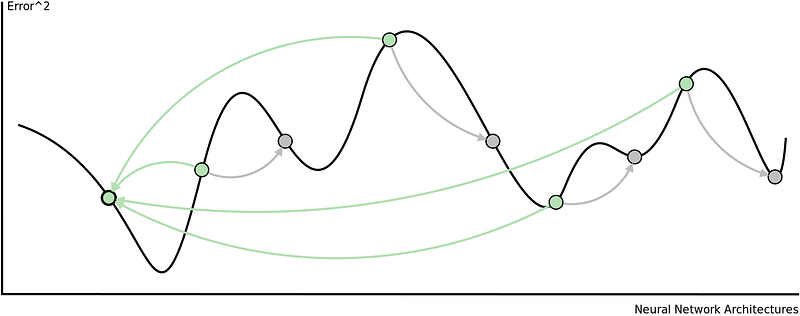
The are some problems with this approach. Adjusting all the weights at once can result in a significant movement of the neural network in weight space, the gradient descent algorithm is quite slow, and the gradient descent algorithm is susceptible to local minima. Local minima are a problem for specific types of neural networks including all product link neural networks. The first two problems can be addressed by using variants of gradient descent including momentum gradient descent (QuickProp), Nesterov’s Accelerated Momentum (NAG) gradient descent, the Adaptive Gradient Algorithm(AdaGrad), Resilient Propagation (RProp), and Root Mean Squared Propagation (RMSProp). As can be seen from the image below, significant improvements can be made on the classical gradient descent algorithm.
That said, these algorithms cannot overcome local minima and are also less useful when trying to optimize both the architecture and weights of a neural network concurrently. To achieve this, global optimization algorithms are needed. Two popular global optimization algorithms are Particle Swarm Optimization (PSO) and Genetic Algorithm (GA). Here is how they can be used to train neural networks.
Neural Network Vector Representation
This is done by encoding the neural network as a vector of weights, each representing the weight of a connection in the neural network. We can train neural networks using most meta-heuristic search algorithms. This technique does not work well with deep neural networks because the vectors become too large.
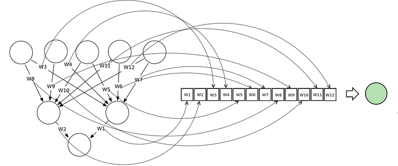
This diagram illustrates how a neural network can be represented in a vector notation and related to the concept of a search space or fitness landscape.
Particle Swarm Optimization
To train a neural network using a PSO, we construct a population/swarm of those neural networks. Each neural network is represented as a vector of weights and is adjusted according to its position from the global best particle and its personal best.
The fitness function is calculated as the sum-squared error of the reconstructed neural network after completing one feedforward pass of the training dataset. The main consideration with this approach is the velocity of the weight updates. This is because if the weights are adjusted too quickly, the sum-squared error of the neural networks will stagnate and no learning will occur.
This diagram shows how particles are attracted to one another in a single swarm Particle Swarm Optimization algorithm.
Genetic Algorithm
To train a neural network using a genetic algorithm, we first construct a population of the vector represented neural networks. Then, we apply the three genetic operators on that population to evolve better and better neural networks. These three operators are:
- Selection: Using the sum-squared error of each network calculated after one feedforward pass, we rank the population of neural networks. The top x% of the population is selected to "survive" to the next generation and be used for crossover.
- Crossover: The top x% of the population’s genes are allowed to cross over with one another. This process forms "offspring." In context, each offspring will represent a new neural network with weights from both of the "parent" neural networks.
- Mutation: This operator is required to maintain genetic diversity in the population. A small percentage of the population are selected to undergo mutation. Some of the weights in these neural networks will be adjusted randomly within a particular range.
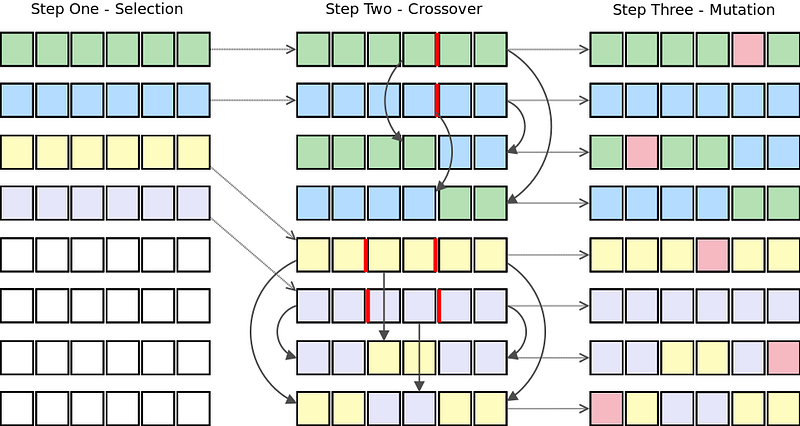
This algorithm shows the selection, crossover, and mutation genetic operators being applied to a population of neural networks represented as vectors.
In addition to these population-based metaheuristic search algorithms, other algorithms have been used to train of neural networks including backpropagation with added momentum, differential evolution, Levenberg Marquardt, simulated annealing, and many more. Personally, I would recommend using a combination of local and global optimization algorithms to overcome the shortcomings of both.
Neural Networks Do Not Always Require a Lot of Data
Neural networks can use one of three learning strategies — namely, a supervised learning strategy, unsupervised learning strategy, or reinforcement learning strategy. Supervised learning requires at least two datasets, a training set that consists of inputs with the expected output, and a testing set that consists of inputs without the expected output. Both of these datasets must consist of labeled data, i.e. data patterns for which the target is known upfront. Unsupervised learning strategies are typically used to discover hidden structures (such as hidden Markov chains) in unlabeled data. They behave in a similar way to clustering algorithms. Reinforcement learning is based on the simple premise of rewarding neural networks for good behaviors and punishing them for bad behaviors. Because unsupervised and reinforcement learning strategies do not require that data be labeled they can be applied to under-formulated problems where the correct output is not known.
Unsupervised Learning
One of the most popular unsupervised neural network architectures is the Self-Organizing Map (also known as the Kohonen Map). Self-Organizing Maps are essentially a multi-dimensional scaling technique which constructs an approximation of the probability density function of some underlying dataset, Z, while preserving the topological structure of that dataset. This is done by mapping input vectors, zi, in the data set, Z, to weight vectors, vj, (neurons) in the feature map, V. Preserving the topological structure simply means that if two input vectors are close together in Z, then the neurons to which those input vectors map in V will also be close together.
For more information on Self-Organizing Maps and how they can be used to produce lower-dimensionality data sets click here. Another interesting application of SOMs is in coloring time series charts for stock trading. This is done to show what the market conditions are at that point in time. This website provides a detailed tutorial and code snippets for implementing the idea for improved Forex trading strategies.
Reinforcement Learning
Reinforcement learning strategies consist of three components. A policy that specifies how the neural network will make decisions, e.g. using technical and fundamental indicators. A reward function that distinguishes good from bad, e.g. making vs. losing money. And a value function which specifies the long term goal. In the context of financial markets (and gameplaying), reinforcement learning strategies are particularly useful because the neural network learns to optimize a particular quantity such as an appropriate measure of risk adjusted return.
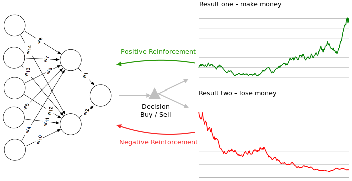
This diagram shows how a neural network can be either negatively or positively reinforced.
PUBLISHED BY : JAYESH BAPU AHIRE
No comments:
Post a Comment