This is related to all the knowledge related with programming, tech news, machine learning, artificial intelligence and news related with development of algorithms, etc
After 6 Years, GIMP 2.10 is Here With Ravishing New Looks and Tons of New Features
BY: Abhishek Prakash
Brief: 6 years after the release of GIMP 2.8, the major new stable release 2.10 is here. Have a look at the new look, new features and installation procedure.
Free and open source image editing application GIMP has a new major release today. GIMP 2.10 comes six years after the last major release 2.8.
It won’t be an exaggeration if I say that GIMP is the most popular image editor in Linux world and perhaps the best Adobe Photoshop alternative. The project was first started in 1996 and in the last 22 years, it has become the default image editor on almost all major Linux distributions. It is also available on Windows and macOS.
What’s new in GIMP 2.10
GIMP 2.10 has been ported to GEGL image processing engine and that’s the biggest change in this release. It brings out several new tools and improvements.
I have been waiting for GIMP 2.10 release for some months now and I am looking forward to using its new features. How about you? Do you use GIMP? What new features you liked in GIMP 2.10?
Many Training Algorithms Exist for Neural Networks
The learning algorithm of a neural network tries to optimize the neural network’s weights until some stopping condition has been met. This condition is typically either when the error of the network reaches an acceptable level of accuracy on the training set, when the error of the network on the validation set begins to deteriorate, or when the specified computational budget has been exhausted. The most common learning algorithm for neural networks is back-propagation, an algorithm that uses stochastic gradient descent, which was discussed earlier on in this series. Backpropagation consists of two steps:
Feed-forward pass: The training dataset is passed through the network and the output from the neural network is recorded and the error of the network is calculated.
Backward propagation: The error signal is passed back through the network and the weights of the neural network are optimized using gradient descent.
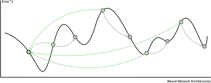
The are some problems with this approach. Adjusting all the weights at once can result in a significant movement of the neural network in weight space, the gradient descent algorithm is quite slow, and the gradient descent algorithm is susceptible to local minima. Local minima are a problem for specific types of neural networks including all product link neural networks. The first two problems can be addressed by using variants of gradient descent including momentum gradient descent (QuickProp), Nesterov’s Accelerated Momentum (NAG) gradient descent, the Adaptive Gradient Algorithm(AdaGrad), Resilient Propagation (RProp), and Root Mean Squared Propagation (RMSProp). As can be seen from the image below, significant improvements can be made on the classical gradient descent algorithm.
That said, these algorithms cannot overcome local minima and are also less useful when trying to optimize both the architecture and weights of a neural network concurrently. To achieve this, global optimization algorithms are needed. Two popular global optimization algorithms are Particle Swarm Optimization (PSO) and Genetic Algorithm (GA). Here is how they can be used to train neural networks.
Neural Network Vector Representation
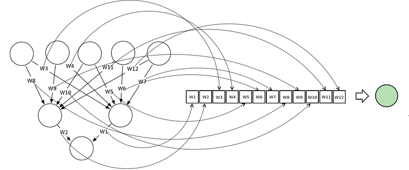
This is done by encoding the neural network as a vector of weights, each representing the weight of a connection in the neural network. We can train neural networks using most meta-heuristic search algorithms. This technique does not work well with deep neural networks because the vectors become too large.
This diagram illustrates how a neural network can be represented in a vector notation and related to the concept of a search space or fitness landscape.
Particle Swarm Optimization
To train a neural network using a PSO, we construct a population/swarm of those neural networks. Each neural network is represented as a vector of weights and is adjusted according to its position from the global best particle and its personal best.
The fitness function is calculated as the sum-squared error of the reconstructed neural network after completing one feedforward pass of the training dataset. The main consideration with this approach is the velocity of the weight updates. This is because if the weights are adjusted too quickly, the sum-squared error of the neural networks will stagnate and no learning will occur.
This diagram shows how particles are attracted to one another in a single swarm Particle Swarm Optimization algorithm.
Genetic Algorithm
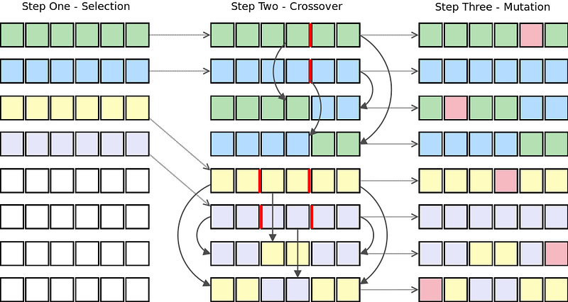
To train a neural network using a genetic algorithm, we first construct a population of the vector represented neural networks. Then, we apply the three genetic operators on that population to evolve better and better neural networks. These three operators are:
Selection: Using the sum-squared error of each network calculated after one feedforward pass, we rank the population of neural networks. The top x% of the population is selected to "survive" to the next generation and be used for crossover.
Crossover: The top x% of the population’s genes are allowed to cross over with one another. This process forms "offspring." In context, each offspring will represent a new neural network with weights from both of the "parent" neural networks.
Mutation: This operator is required to maintain genetic diversity in the population. A small percentage of the population are selected to undergo mutation. Some of the weights in these neural networks will be adjusted randomly within a particular range.
This algorithm shows the selection, crossover, and mutation genetic operators being applied to a population of neural networks represented as vectors.
In addition to these population-based metaheuristic search algorithms, other algorithms have been used to train of neural networks including backpropagation with added momentum, differential evolution, Levenberg Marquardt, simulated annealing, and many more. Personally, I would recommend using a combination of local and global optimization algorithms to overcome the shortcomings of both.
Neural Networks Do Not Always Require a Lot of Data
Neural networks can use one of three learning strategies — namely, a supervised learning strategy, unsupervised learning strategy, or reinforcement learning strategy. Supervised learning requires at least two datasets, a training set that consists of inputs with the expected output, and a testing set that consists of inputs without the expected output. Both of these datasets must consist of labeled data, i.e. data patterns for which the target is known upfront. Unsupervised learning strategies are typically used to discover hidden structures (such as hidden Markov chains) in unlabeled data. They behave in a similar way to clustering algorithms. Reinforcement learning is based on the simple premise of rewarding neural networks for good behaviors and punishing them for bad behaviors. Because unsupervised and reinforcement learning strategies do not require that data be labeled they can be applied to under-formulated problems where the correct output is not known.
Unsupervised Learning
One of the most popular unsupervised neural network architectures is the Self-Organizing Map (also known as the Kohonen Map). Self-Organizing Maps are essentially a multi-dimensional scaling technique which constructs an approximation of the probability density function of some underlying dataset, Z, while preserving the topological structure of that dataset. This is done by mapping input vectors, zi, in the data set, Z, to weight vectors, vj, (neurons) in the feature map, V. Preserving the topological structure simply means that if two input vectors are close together in Z, then the neurons to which those input vectors map in V will also be close together.
For more information on Self-Organizing Maps and how they can be used to produce lower-dimensionality data sets click here. Another interesting application of SOMs is in coloring time series charts for stock trading. This is done to show what the market conditions are at that point in time. This website provides a detailed tutorial and code snippets for implementing the idea for improved Forex trading strategies.
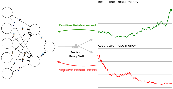
Reinforcement Learning
Reinforcement learning strategies consist of three components. A policy that specifies how the neural network will make decisions, e.g. using technical and fundamental indicators. A reward function that distinguishes good from bad, e.g. making vs. losing money. And a value function which specifies the long term goal. In the context of financial markets (and gameplaying), reinforcement learning strategies are particularly useful because the neural network learns to optimize a particular quantity such as an appropriate measure of risk adjusted return.
This diagram shows how a neural network can be either negatively or positively reinforced.
Half a century ago, the pioneers of chaos theory discovered that the “butterfly effect” makes long-term prediction impossible. Even the smallest perturbation to a complex system (like the weather, the economy or just about anything else) can touch off a concatenation of events that leads to a dramatically divergent future. Unable to pin down the state of these systems precisely enough to predict how they’ll play out, we live under a veil of uncertainty.
But now the robots are here to help.
In a series of results reported in the journals Physical Review Letters and Chaos, scientists have used machine learning — the same computational technique behind recent successes in artificial intelligence — to predict the future evolution of chaotic systems out to stunningly distant horizons. The approach is being lauded by outside experts as groundbreaking and likely to find wide application.
“I find it really amazing how far into the future they predict” a system’s chaotic evolution, said Herbert Jaeger, a professor of computational science at Jacobs University in Bremen, Germany.
The findings come from veteran chaos theorist Edward Ott and four collaborators at the University of Maryland. They employed a machine-learning algorithm called reservoir computing to “learn” the dynamics of an archetypal chaotic system called the Kuramoto-Sivashinsky equation. The evolving solution to this equation behaves like a flame front, flickering as it advances through a combustible medium. The equation also describes drift waves in plasmas and other phenomena, and serves as “a test bed for studying turbulence and spatiotemporal chaos,” said Jaideep Pathak, Ott’s graduate student and the lead author of the new papers.
After training itself on data from the past evolution of the Kuramoto-Sivashinsky equation, the researchers’ reservoir computer could then closely predict how the flamelike system would continue to evolve out to eight “Lyapunov times” into the future, eight times further ahead than previous methods allowed, loosely speaking. The Lyapunov time represents how long it takes for two almost-identical states of a chaotic system to exponentially diverge. As such, it typically sets the horizon of predictability.
“This is really very good,” Holger Kantz, a chaos theorist at the Max Planck Institute for the Physics of Complex Systems in Dresden, Germany, said of the eight-Lyapunov-time prediction. “The machine-learning technique is almost as good as knowing the truth, so to say.”
The algorithm knows nothing about the Kuramoto-Sivashinsky equation itself; it only sees data recorded about the evolving solution to the equation. This makes the machine-learning approach powerful; in many cases, the equations describing a chaotic system aren’t known, crippling dynamicists’ efforts to model and predict them. Ott and company’s results suggest you don’t need the equations — only data. “This paper suggests that one day we might be able perhaps to predict weather by machine-learning algorithms and not by sophisticated models of the atmosphere,” Kantz said.
Besides weather forecasting, experts say the machine-learning technique could help with monitoring cardiac arrhythmias for signs of impending heart attacks and monitoring neuronal firing patterns in the brain for signs of neuron spikes. More speculatively, it might also help with predicting rogue waves, which endanger ships, and possibly even earthquakes.
Ott particularly hopes the new tools will prove useful for giving advance warning of solar storms, like the one that erupted across 35,000 miles of the sun’s surface in 1859. That magnetic outburst created aurora borealis visible all around the Earth and blew out some telegraph systems, while generating enough voltage to allow other lines to operate with their power switched off. If such a solar storm lashed the planet unexpectedly today, experts say it would severely damage Earth’s electronic infrastructure. “If you knew the storm was coming, you could just turn off the power and turn it back on later,” Ott said.
He, Pathak and their colleagues Brian Hunt, Michelle Girvan and Zhixin Lu (who is now at the University of Pennsylvania) achieved their results by synthesizing existing tools. Six or seven years ago, when the powerful algorithm known as “deep learning” was starting to master AI tasks like image and speech recognition, they started reading up on machine learning and thinking of clever ways to apply it to chaos. They learned of a handful of promising results predating the deep-learning revolution. Most importantly, in the early 2000s, Jaeger and fellow German chaos theorist Harald Haas made use of a network of randomly connected artificial neurons — which form the “reservoir” in reservoir computing — to learn the dynamics of three chaotically coevolving variables. After training on the three series of numbers, the network could predict the future values of the three variables out to an impressively distant horizon. However, when there were more than a few interacting variables, the computations became impossibly unwieldy. Ott and his colleagues needed a more efficient scheme to make reservoir computing relevant for large chaotic systems, which have huge numbers of interrelated variables. Every position along the front of an advancing flame, for example, has velocity components in three spatial directions to keep track of.
It took years to strike upon the straightforward solution. “What we exploited was the locality of the interactions” in spatially extended chaotic systems, Pathak said. Locality means variables in one place are influenced by variables at nearby places but not by places far away. “By using that,” Pathak explained, “we can essentially break up the problem into chunks.” That is, you can parallelize the problem, using one reservoir of neurons to learn about one patch of a system, another reservoir to learn about the next patch, and so on, with slight overlaps of neighboring domains to account for their interactions.
Parallelization allows the reservoir computing approach to handle chaotic systems of almost any size, as long as proportionate computer resources are dedicated to the task.
Ott explained reservoir computing as a three-step procedure. Say you want to use it to predict the evolution of a spreading fire. First, you measure the height of the flame at five different points along the flame front, continuing to measure the height at these points on the front as the flickering flame advances over a period of time. You feed these data-streams in to randomly chosen artificial neurons in the reservoir. The input data triggers the neurons to fire, triggering connected neurons in turn and sending a cascade of signals throughout the network.
The second step is to make the neural network learn the dynamics of the evolving flame front from the input data. To do this, as you feed data in, you also monitor the signal strengths of several randomly chosen neurons in the reservoir. Weighting and combining these signals in five different ways produces five numbers as outputs. The goal is to adjust the weights of the various signals that go into calculating the outputs until those outputs consistently match the next set of inputs — the five new heights measured a moment later along the flame front. “What you want is that the output should be the input at a slightly later time,” Ott explained.
To learn the correct weights, the algorithm simply compares each set of outputs, or predicted flame heights at each of the five points, to the next set of inputs, or actual flame heights, increasing or decreasing the weights of the various signals each time in whichever way would have made their combinations give the correct values for the five outputs. From one time-step to the next, as the weights are tuned, the predictions gradually improve, until the algorithm is consistently able to predict the flame’s state one time-step later.
“In the third step, you actually do the prediction,” Ott said. The reservoir, having learned the system’s dynamics, can reveal how it will evolve. The network essentially asks itself what will happen. Outputs are fed back in as the new inputs, whose outputs are fed back in as inputs, and so on, making a projection of how the heights at the five positions on the flame front will evolve. Other reservoirs working in parallel predict the evolution of height elsewhere in the flame.
In a plot in their PRL paper, which appeared in January, the researchers show that their predicted flamelike solution to the Kuramoto-Sivashinsky equation exactly matches the true solution out to eight Lyapunov times before chaos finally wins, and the actual and predicted states of the system diverge.
The usual approach to predicting a chaotic system is to measure its conditions at one moment as accurately as possible, use these data to calibrate a physical model, and then evolve the model forward. As a ballpark estimate, you’d have to measure a typical system’s initial conditions 100,000,000 times more accurately to predict its future evolution eight times further ahead.
That’s why machine learning is “a very useful and powerful approach,” said Urlich Parlitz of the Max Planck Institute for Dynamics and Self-Organization in Göttingen, Germany, who, like Jaeger, also applied machine learning to low-dimensional chaotic systems in the early 2000s. “I think it’s not only working in the example they present but is universal in some sense and can be applied to many processes and systems.” In a paper soon to be published in Chaos, Parlitz and a collaborator applied reservoir computing to predict the dynamics of “excitable media,” such as cardiac tissue. Parlitz suspects that deep learning, while being more complicated and computationally intensive than reservoir computing, will also work well for tackling chaos, as will other machine-learning algorithms. Recently, researchers at the Massachusetts Institute of Technology and ETH Zurich achieved similar results as the Maryland team using a “long short-term memory” neural network, which has recurrent loops that enable it to store temporary information for a long time.
Since the work in their PRL paper, Ott, Pathak, Girvan, Lu and other collaborators have come closer to a practical implementation of their prediction technique. In new research accepted for publication inChaos, they showed that improved predictions of chaotic systems like the Kuramoto-Sivashinsky equation become possible by hybridizing the data-driven, machine-learning approach and traditional model-based prediction. Ott sees this as a more likely avenue for improving weather prediction and similar efforts, since we don’t always have complete high-resolution data or perfect physical models. “What we should do is use the good knowledge that we have where we have it,” he said, “and if we have ignorance we should use the machine learning to fill in the gaps where the ignorance resides.” The reservoir’s predictions can essentially calibrate the models; in the case of the Kuramoto-Sivashinsky equation, accurate predictions are extended out to 12 Lyapunov times.
The duration of a Lyapunov time varies for different systems, from milliseconds to millions of years. (It’s a few days in the case of the weather.) The shorter it is, the touchier or more prone to the butterfly effect a system is, with similar states departing more rapidly for disparate futures. Chaotic systems are everywhere in nature, going haywire more or less quickly. Yet strangely, chaos itself is hard to pin down. “It’s a term that most people in dynamical systems use, but they kind of hold their noses while using it,” said Amie Wilkinson, a professor of mathematics at the University of Chicago. “You feel a bit cheesy for saying something is chaotic,” she said, because it grabs people’s attention while having no agreed-upon mathematical definition or necessary and sufficient conditions. “There is no easy concept,” Kantz agreed. In some cases, tuning a single parameter of a system can make it go from chaotic to stable or vice versa.
Wilkinson and Kantz both define chaos in terms of stretching and folding, much like the repeated stretching and folding of dough in the making of puff pastries. Each patch of dough stretches horizontally under the rolling pin, separating exponentially quickly in two spatial directions. Then the dough is folded and flattened, compressing nearby patches in the vertical direction. The weather, wildfires, the stormy surface of the sun and all other chaotic systems act just this way, Kantz said. “In order to have this exponential divergence of trajectories you need this stretching, and in order not to run away to infinity you need some folding,” where folding comes from nonlinear relationships between variables in the systems.
The stretching and compressing in the different dimensions correspond to a system’s positive and negative “Lyapunov exponents,” respectively. In another recent paper in Chaos, the Maryland team reported that their reservoir computer could successfully learn the values of these characterizing exponents from data about a system’s evolution. Exactly why reservoir computing is so good at learning the dynamics of chaotic systems is not yet well understood, beyond the idea that the computer tunes its own formulas in response to data until the formulas replicate the system’s dynamics. The technique works so well, in fact, that Ott and some of the other Maryland researchers now intend to use chaos theory as a way to better understand the internal machinations of neural network.
This algorithm automatically spots “face swaps” in videos
But the same system can be used to make better fake videos that are harder to detect.
by Emerging Technology from the arXiv
April 10, 2018
The ability to take one person’s face or expression and superimpose it onto a video of another person has recently become possible. In particular, pornographic videos called “deepfakes” have emerged on websites such as Reddit and 4Chan showing famous individuals’ faces superimposed onto the bodies of actors.
This phenomenon has significant implications. At the very least, it has the potential to undermine the reputation of people who are victims of this kind of forgery. It poses problems for biometric ID systems. And it threatens to undermine public trust in videos of any kind.
So a quick and accurate way to spot these videos is desperately needed.
Which of these pairs of images are forgeries? Answer below.
Enter Andreas Rossler at the Technical University of Munich in Germany and colleagues, who have developed a deep-learning system that can automatically spot face-swap videos. The new technique could help identify forged videos as they are posted to the web.
But the work also has sting in the tail. The same deep-learning technique that can spot face-swap videos can also be used to improve the quality of face swaps in the first place—and that could make them harder to detect.
The new technique relies on a deep-learning algorithm that Rossler and co have trained to spot face swaps. These algorithms can only learn from huge annotated data sets of good examples, which simply have not existed until now.
So the team began by creating a large data set of face-swap videos and their originals. They use two types of face swaps that can be easily made using software called Face2Face. (This software was created by some members of this team.)
The team have done this with over 1,000 videos, creating a database of about half a million images in which the faces have been manipulated with state-of-the-art face-editing software. They called this the FaceForensics database.The first type of face swap superimposes one person’s face on another’s body so that it takes on their expressions. The second takes the expressions from one face and modifies a second face to show them.
The size of this database is a significant improvement over what had been previously available. “We introduce a novel data set of manipulated videos that exceeds all existing publicly available forensic data sets by orders of magnitude,” says Rossler and co.
Next, the team uses the database to train a deep-learning algorithm to recognize the difference between face swaps and their unadulterated originals. They call the resulting algorithm XceptionNet.
Finally, they compare the new approach to other forgery detection techniques.
The results are impressive. XceptionNet clearly outperforms other techniques in spotting videos that have been manipulated, even when the videos have been compressed, which makes the task significantly harder. “We set a strong baseline of results for detecting a facial manipulation with modern deep-learning architectures,” say Rossler and co.
That should make it easier to spot forged videos as they are uploaded to the web. But the team is well aware of the cat-and-mouse nature of forgery detection: as soon as a new detection technique emerges, the race begins to find a way to fool it.
Rossler and co have a natural head start since they developed XceptionNet. So they use it to spot the telltale signs that a video has been manipulated and then use this information to refine the forgery, making it even harder to detect.
It turns out that this process improves the visual quality of the forgery but does not have much effect on XceptionNet’s ability to detect it. “Our refiner mainly improves visual quality, but it only slightly encumbers forgery detection for deep-learning method trained exactly on the forged output data,” they say.
That’s interesting work since it introduces an entirely new way of improving the process of image manipulation. “We believe that this interplay between tampering and detection is an extremely exciting avenue for follow-up work,” they say.


